Monte Carlo Simulations in Statistical Physics Classical interacting - PowerPoint PPT Presentation

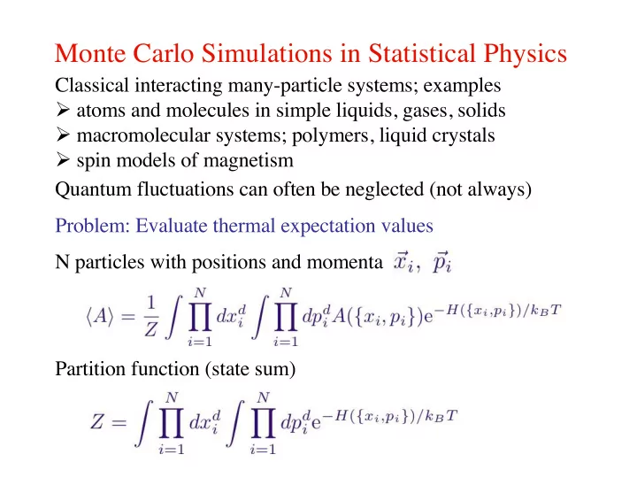
Monte Carlo Simulations in Statistical Physics Classical interacting many-particle systems; examples Ø atoms and molecules in simple liquids, gases, solids Ø macromolecular systems; polymers, liquid crystals Ø spin models of magnetism Quantum fluctuations can often be neglected (not always) Problem: Evaluate thermal expectation values N particles with positions and momenta Partition function (state sum)

Hamiltonian (energy function) for identical particles in potential U and with pair-interaction V If the observable A is velocity-independent (real-space correlation functions, response of local density to external perturbations, etc.), the momentum integrals cancel Only the potential energy matters

For the kinetic energy the position integrals cancel This gives the equipartition theorem Most of statistical physics concerns velocity-independent quantities; the mathematical problem of interest is With N approaching infinity (thermodynamic limit) Few exact solutions; numerical simulations for finite N important

Lattice and spin models Degrees of fredom “ live ” on vertices of a lattice Ø Continuous or discrete variables on the vertices Spin models, describing magnetism of solids with spinful atoms Ø large spin S behaves as classical angular momentum Ø quantum fluctuations important for small S (1/2,1,3/2) Interactions: often of the Heisenberg form

Ising models Two states on each lattice site Can arise for quantum mechanical S=1/2: Strong anisotropies; z-interactions can dominate This is the Ising model Ø important in the theory of magnetism Ø also effective model for other stat mech problems ( “ lattice gases ” , binary alloys, atom adsorption on surfaces,...) With only nearest-neighbor interactions (J), the Ising model can be solved analytically in 1D and 2D Ø Numerical simulations important in most other cases

Two-dimensional Ising model denotes nearest neighbors Ferromagnetic or antiferromagnetic ground state (T=0) Related by transformation: on one sublattice Thermal expectation value of some quantity A

Phase transition Spontaneous ordering (symmetry breaking) at critical temperature √ magnetization (ferromagnet) T c /J = 2 / ln(1 + 2) sublattice (staggered) magnetization (antiferromagnet)