Monte Carlo simulation of the 2D Ising model - tutorial - Zoltn Nda - PowerPoint PPT Presentation
Monte Carlo simulation of the 2D Ising model - tutorial - Zoltn Nda Babe-Bolyai University Department of Theoretical and Computational Physics . A basic Metropolis Algorithm for simulating the 2D and 3D Ising model on square lattice
Monte Carlo simulation of the 2D Ising model - tutorial - Zoltán Néda Babeş-Bolyai University Department of Theoretical and Computational Physics . A basic Metropolis Algorithm for simulating the 2D and 3D ١ Ising model on square lattice free boundary condition ٢ . Implementing the periodic boundary condition ٣ . Calculating averages as a function of temperature. Finite- size effects. Calculation of: m ( T ) C V ( T ) ( T )
The Ising model H J S S h S i j i i , j { i } S ١ i we fix J=1 k=1 fixing the units for T h=0 no external magnetic field - spontaneous magnetization is possible (M 0 for h=0) - first model for understanding ferro- and anti-ferromagnetism for localized spins encoded in a Matrix M[X][Y] ( DimX x DimY) - for J>0 --> ferromagnetic order - for J<0 --> anti-ferromagnetic order M [ X ][ Y ] S ١ i - no phase transition in 1D S ١ - ferro-paramagnetic phase transition for D>1 i - second order phase transition S ١ (order-disorder) i
The Metropolis algorithm: Single spin-flip algorithm one spin with coordinates (X=I, Y=j) is attempted to flip exp[ E ( x , x ' )] for E ( x , x ' ) ٠ P P ( x x ' ) ١ for E ( x , x ' ) ٠ S M [ i ][ j ] initial S M [ i ][ j ] final i , j E M [ i ][ j ] { M [ i ١ ][ j ] M [ i ١ ][ j ] M [ i ][ j ١ ] M [ i ][ j ١ ]} initial i , j E M [ i ][ j ] { M [ i ١ ][ j ] M [ i ١ ][ j ] M [ i ][ j ١ ] M [ i ][ j ١ ]} final i , j i , j E E E ٢ * M [ i ][ j ] * { M [ i ١ ][ j ] M [ i ١ ][ j ] M [ i ][ j ١ ] M [ i ][ j ١ ]} final initial Spins are randomly selected and flipped with a P probability Mag M [ x ][ y ] x ١ , DimX after the transient (“heat-up”) steps the magnetization y ١ , DimY (Mag) and total energy (E) is followed in time (MC m Mag /( DimX DimY ) steps) ١ E M [ x ][ y ] { M [ x ١ ][ y ] M [ x ١ ][ y ] M [ x ][ y ١ ] M [ x ][ y ١ ]} ٢ x ١ , DimX y ١ , DimY
The Metropolis MC algorithm for the problem: 1. Fix a temperature (T) i ١ , N ١ { } 2. Consider an initial spin configuration ( ). For example for all i i 3. Calculate the initial value of E and M 4 . Consider a new spin configuration by virtually “flipping” one randomly selected spin E 5 . Calculate the energy E’ of the new configuration, and the energy change due to this spin-flip 6. Calculate the Metropolis P=P(x-->x’) probabilities for this change 7 . Generate a random number “r” between 0 and 1 r P 8. If accept the flip and update the value of the energy to E’ and magnetization to M’ r P If reject the spin flip and take again the initial E and M values in the needed averages 9. Repeat the steps 4 - 8 many times (drive the system to the desired canonical distribution of the states) 10. Repeat the steps 4 -8 by collecting the values of E, E 2 , M, M 2 , for the needed averages 11. Compute this average for a large number of microstates 12. Calculate the value of m(T), <E(T)>, C v (T) and (T) using the given formulas 13. Change the temperature and repeat the algorithm for the new temperatures as well. 14. Construct the desired m(T), <E(T)>, C v (T), (T) curves
1. Basic program for free boundary condition Free boundary condition realized by adding a extra rows and columns to the boundaries and considering there spins with S=0 spins! this gives no contribution to the energies fixing the parameters boundary() flowchart of a init( ) fixing the free boundary condition by basic C program M[0][i]=M[DimX+1][i]=0 -initializes M[X][Y] randomly M[i][0]=M[i][DimY+1]=0 -initializes boundaries int ram(i) MC steps =0 randomly select one spin generate a random yes float between [0,1) no flip( ) randf( ) ii<Configurations flip the selected spin with generate a Metropolis probability random integer pconf() no use program isinga.c print on the screen the spin count MC steps configuration (S=1 1; S=-1 Understand the program, 0) If MC steps=MCw run-it and modify for 3D i++; yes
some Linux commands - to go in the working directory cd zneda - to see what is there ls -l - editing the code: gedit isinga.c or kedit isinga.c -compiling the code cc isinga.c –lm –o isinga -running the code ./isinga -plotting the results xmgrace magn.dat or gnuplot >p ‘magn.dat’ u 1:3 w lp (this gnuplot instruction plots from file “magn.dat” the third column as a function of the first, with line-connected points)
2. Basic program for periodic boundary condition The periodic boundary conditions are realized by adding a extra rows and columns to the boundaries, copying the last (first) row (column). See the picture: original spin matrix extra rows and columns of spins Important! when a spin at the boundaries is flipped, it’s image in the added rows (columns) have to be also flipped! use program isingb.c Understand the code, run-it and modify it for 3D
3. Calculating averages as a function of temperature. Finite-size effects. Calculation of: m ( T ) C V ( T ) ( T ) -The system is “heated-up” i and no averages are i M i i m ( T ) calculated for Step_trans N N N MC steps. -The <m>,<M>, <M 2 >, <E> and ١ ٢ ٢ ( T ) M ( T ) M ( T ) <E 2 > averages are computed NT for Step_max MC steps - Results are written out in ١ ٢ ٢ C v ( T ) E ( T ) E ( T ) the “magn.dat” file! ٢ NT use program isingc.c - Understand it, run it, modify it for 3D. - Change the system size, and study finite-size effects! m ( T ) C V ( T ) ( T ) -Plot the desired curves -Study finite-size effects
Recommend
More recommend
Explore More Topics
Stay informed with curated content and fresh updates.

