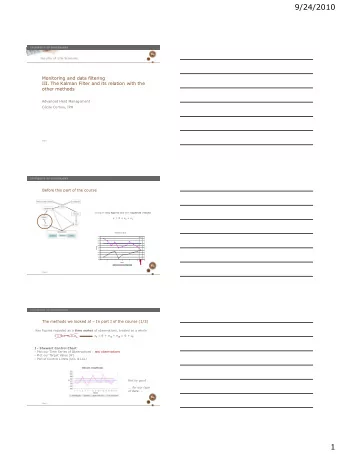
Monitoring and data filtering III. The Kalman Filter and its - PowerPoint PPT Presentation

Monitoring and data filtering III. The Kalman Filter and its relation with the other methods Advanced Quantitative Herd Management Dan Jensen, IPH Dias 1

Before this part of the course Compare key figures (k) with expected results κ = θ + e s + e o Results from 2 herds 880 870 860 850 840 Gain (g) 830 820 810 800 790 780 0 2 4 6 8 10 12 Quarter Expected Herd A Herd B Dias 2

The methods we looked at – In part I of the course (1/3) Key figures regarded as a time series of observations, treated as a whole κ = θ + e s + e o κ t = θ + e s t + e o t = θ + v t I - Shewart Control Chart - Plot our Time Series of Observations : raw observations - Plot our Target Value (θ’) - Plot of Control Limits (UCL & LCL) Not so good ... for our type of data ... Dias 3

The methods we looked at – In part I of the course (2/3) II - Shewart Control Chart III - Shewart Control Chart - Plot an EWMA of our observations - Plot a Moving Average of observations - Plot our Target Value (θ’) - Plot our Target Value (θ’) - Plot of Control Limits (UCL & LCL) - Plot of Control Limits (UCL & LCL) Still not so good Here: milk yield ... for our type of data Dias 4

The methods we looked at – In part I of the course (3/3) IV – Autocorrelated data V – EWMA for autocorrelated data - Use EWMA as one-step-ahead - Model the data predictor - Calculate a prediction for next obs. - Plot the prediction errors - Plot the prediction errors Here we use 0 as Center Line and see how error terms are distributed Dias 5

The methods we looked at – In part II of the course (1/4) Before: κ t = θ + e s t + e o t = θ + v t A Simple DLM Time series Y t = (y 1 , ... , y n ) Observation equation: θ t + v t , v t » N(0, V t ) y t = θ θ θ Like before: v t = e s + e o The symbol θ θ t is the underlying true value at time t . θ θ System equation: θ t -1 + w t , w t » N(0, W t ) θ θ θ θ t = θ θ θ The true value is not any longer assumed to be constant . Dias 6

The methods we looked at – In part II of the course (2/4) The Kalman Filter ( µ t-1 | D t-1 ) » N(m t-1 , C t-1 ) ( µ t | D t ) » N(m t , C t ) The updating equations of the Kalman Filter are used for stepwise calculation of m t and C t DLM and EWMA DLM EWMA ( 1 ) ( 1 ) = + − = λκ + − λ m A Y A m z z − 1 1 t t t t t − t t t As the model adapts to the data, A t converges and becomes A The calculation of the mean of the underlying level for the simple DLM looks very similar to the calculation of the EWMA Dias 7

The methods we looked at – In part II of the course (3/4) The different models - Simple DLM - DLM with a trend General form of the DLM Observation Equation: Y t = F’ t θ t + ν t , ν t ~ N(0,V t ) System Equation: θ t = G t θ t-1 + ω t , ω t ~ N(0,W t ) θ t = ( θ 1 , … , θ m )’ is a vector of parameters describing the system at time t. Can include: Level, Trend, + External information Structure Seasonality, Periodicity, ... According to the data observed, the use of DLM allows many modeling possibilities Dias 8

The methods we looked at – In part II of the course (4/4) Monitoring methods used with DLM Monitor the forecast errors (e t = Y t – f t ) as we did with autocorrelated data in part I NO need for ’expected value’ V-mask (cusum) alarm limits Can look at the different components of the models (trends, seasons) Dias 9

The multi process kalman filter (MPKF) (1/2) Multi Process Models Class I ex: Classifying sows activities in Farrowing house A single out of a range of possible DLMs is viewed as appropriate at all time for describing the entire time series Parameters : V and W � We try to find out which model is it at time t? Dias 10

The multi process kalman filter (MPKF) (2/2) Multi Process Models Class II ex: Monitoring Somatic Cell Counts / Boar visits No single DLM as adequate for all time: the possibility that different models are appropriate at different times is explicitly recognised and modelled through different defining parameters Parameters : V and W and Π (values for Π define fixed prior probabilities) � We try to find out normal evolution, outlier, level shift � We need to go back f.x. two, three steps to check which model is the right one Dias 11

Sum up of sum up We increased the complexity of our models and monitoring methods to try to adapt to the complexity of monitoring living beings Methods here based on a whole time series of observations -> need for automatic registration -> potential on-line monitoring From part I to part II, we made our model dynamics, so the ’true underlying level’ is no more constant Dias 12