Module 7: Introduction to Queueing Theory (Notation, Single Queues, - PowerPoint PPT Presentation
Module 7: Introduction to Queueing Theory (Notation, Single Queues, Littles Result) (Slides based on Daniel A. Reed, ECE/CS 441 Notes, Fall 1995, used with permission) ECE/CS 441: Computer System Analysis Module 6, Slide 1 Outline of Section
Module 7: Introduction to Queueing Theory (Notation, Single Queues, Little’s Result) (Slides based on Daniel A. Reed, ECE/CS 441 Notes, Fall 1995, used with permission) ECE/CS 441: Computer System Analysis Module 6, Slide 1
Outline of Section on Queueing Theory 1. Notation 2. Little’s Result 3. Single Queues 4. Solutions for networks of queues - Product Form Results (on blackboard, not slides) 5. Mean value analysis (if time permits) ECE/CS 441: Computer System Analysis Module 6, Slide 2
Queueing Theory Notation • Queuing characteristics – Arrival process – Service time distribution – Number of servers – System capacity – Population size – Service discipline • Each of these is described mathematically – Descriptions determine tractability of (efficient) analytic solution – Only a small set of possibilities are solvable using standard queueing theory ECE/CS 441: Computer System Analysis Module 6, Slide 3
Arrival Processes • Suppose jobs arrive at times t 1 , t 2 , ... , t j – Random variables τ j = t j - t j -1 are inter-arrival times – There are many possible assumptions for the distribution of the τ j – Typical assumptions for the τ j : • Independent • Identically distributed – Many other possible assumptions: • Bulk arrivals • Balking • Correlated arrivals • For Poisson arrival, the inter-arrival times are: – IID (independent and identically distributed) – exponentially distributed (i.e., CDF F ( x ) = 1 - e - x / a ) • Other common arrival time distributions include – Erlang, Hyper-exponential, Deterministic, General (with a specified mean and variance) ECE/CS 441: Computer System Analysis Module 6, Slide 4
Other Queue Features • Service time – Interval spent actually receiving service (exclusive of waiting time) – As with arrival processes, there are many possible assumptions – Most common assumptions are • IID random variables • exponential service time distribution • Number of servers – Servers may or may not be identical – Service discipline determines allocation of customers to servers • System capacity – Maximum number of customers in the system (including those in service) – May be finite or infinite • Population size – Total number of potential customers – May be finite or infinite ECE/CS 441: Computer System Analysis Module 6, Slide 5
Other Queue Features (Continued) • Service discipline – The order waiting customers are serviced – Many possibilities, including • First-come-first-serve (FCFS), the most common • Last-come-first-serve (LCFS) • Last-come-first-serve preempt resume (LCFS-PR) • Round robin (RR) with finite quantum size • Processor sharing (PS) --- RR with infinitesimal quantum size • Infinite server (IS) – Almost anything might be used, depending on the the total state of the queue – As expected, service discipline affects the nature of the stochastic process that represents the behavior of the queueing system ECE/CS 441: Computer System Analysis Module 6, Slide 6
Queueing Discipline Specification • Queueing discipline is typically specified using Kendall’s notation ( A / S / m / B / K / SD ), where – Letters correspond to six queue attributes • A : interarrival time distribution • S : service time distribution • m : number of servers • B : number of buffers (system capacity) • K : population size • SD : service discipline • Interarrival and service time specifiers – M exponential – E k Erlang with parameter k – H k hyperexponential with parameter k – D deterministic – G general (any distribution, mean and variance used in the solution) • Bulk arrivals or service are denoted by a superscript – M [ x ] denotes exponential arrivals with group size x – x is generally a random variable with separately specified distribution • Omitted specifiers assume certain defaults – infinite buffer capacity – infinite population size – FCFS service discipline ECE/CS 441: Computer System Analysis Module 6, Slide 7
Example Queueing Discipline Specifications • M / D /5/40/200/ FCFS – Exponentially distributed interarrival times – Deterministic service times – Five servers – Forty buffers (35 for waiting) – Total population of 200 customers – First-come-first-serve service discipline • M / M /1 – Exponentially distributed interarrival times – Exponentially distributed service times – One server – Infinite number of buffers – Infinite population size – First-come-first-serve service discipline ECE/CS 441: Computer System Analysis Module 6, Slide 8
An Introductory Example • Given these descriptions, what are examples of their application? • Consider a typical bank – 5 tellers – Customers form a single line and are serviced FCFS – Excluding a run on the bank, the waiting room is effectively infinite – For a large bank, the population is effectively infinite – Bulk arrivals are possible if friends arrive together for service • What about service time and inter-arrival time distributions? – We can go measure them with a watch at the bank – Or, we can make mathematically simplifying assumptions – Latter is most common and exponential distribution is typical • Combining these facts and assumptions – M / M /1 queue – As we shall see, the mean queue length (including one in service) for an M / M /1 queue is ! µ " ! – Where • λ is the mean inter-arrival time • µ is the mean service time ECE/CS 441: Computer System Analysis Module 6, Slide 9
Notation and Basic “Facts” • Standard variable names – τ is job interarrival time – λ = 1/ E [ τ ] mean job arrival rate – s is service time per customer (job) – m is number of servers – µ = 1/ E [ s ] is mean service rate per server – n = n q + n s is number of jobs in the system – n q is number of jobs waiting to receive service – n s is number of jobs in service – r is response time (service time plus queueing delay) – w is waiting time (queueing delay only) • System must be “stable” to have an interesting steady state solution – Number of jobs in the system is finite – Requires the relation λ < m µ hold unless • the population is finite (queue length is bounded) • the buffer capacity is finite (arrivals are lost when queue is full) • (in these cases, system is always stable) ECE/CS 441: Computer System Analysis Module 6, Slide 10
Notation and Basic “Facts” • Number of jobs in the system – n = n q + n s (jobs are either waiting or in service) – E [ n ] = E [ n q ] + E [ n s ] (or n = n q + n s ) – and, if the service rates are independent of queue length • Cov ( n q , n s ) = 0 • Var [ n ] = Var [ n q ] + Var [ n s ] • Number and time – r = w + s (response time is the sum of queueing delay and service) = + – but, r , w , and s are random variables , so r w s – and, if the service rates are independent of queue length • Cov ( w , s ) = 0 • Var [ r ] = Var [ w ] + Var [ s ] ECE/CS 441: Computer System Analysis Module 6, Slide 11
Little’s Law • Very important result -- Part of the queueing folk literature for the past century • Formal proof due to J. D. C. Little (1961) • Relates mean queue length to arrival rate and mean response time • Mathematically (in seady state), n = ! r • Applies to any “black box” queue under the following assumptions – System is work conserving – Number of jobs entering is same as number leaving (system is stable) • Also applies to any transient interval, without requirement that system be stable. • Note that these are very general conditions, and can apply for any system (“black box”) in which customers leave and enter subject to the above constraints. • An intuitive proof... ECE/CS 441: Computer System Analysis Module 6, Slide 12
Little’s Law (Continued) • Sketch of proof (of steady-state case): During a long interval, arrivals ≈ departures (else no stability) – – Area under the curve is total job time units (jobs x time) arrival – Mean queue length is average curve height (area/time) n rate – Mean time in system is area/arrivals r jobs x time jobs x time jobs x = time jobs – Mean arrival rate is arrivals/time time • A very general result: Avg time in system Avg number in system – No assumptions about arrival or service processes – Holds for any queueing discipline (simply charge the area differently) ECE/CS 441: Computer System Analysis Module 6, Slide 13
Analysis of Single Queues • Plan: – Start with one of the simplest queues, an M / M /1 – Model as a “birth-death” process – Generalize result to other types of queues • A birth-death process is a Markov process in which states are numbered a integers, and transitions are only permitted between “neighboring” states. • Steady state solution of a birth death process (Kleinrock, Queueing Systems, vol. 1): – ( Theorem ) steady state probability p n of being in state n is p n = ! 0 ! 1 ... ! n " 1 p 0 n = 1,2,..., # µ 1 µ 2 ... µ n – where p 0 is the probability of being in state 0 • Now for a proof ... ECE/CS 441: Computer System Analysis Module 6, Slide 14
Recommend
More recommend
Explore More Topics
Stay informed with curated content and fresh updates.
