Queueing Networks service to a collection of customers that - PowerPoint PPT Presentation
Queueing Networks Stochastic models of resource sharing systems computer, communication, traffic, manufacturing systems Queueing Network a system model set of service centers representing the system resources that provide Queueing Networks
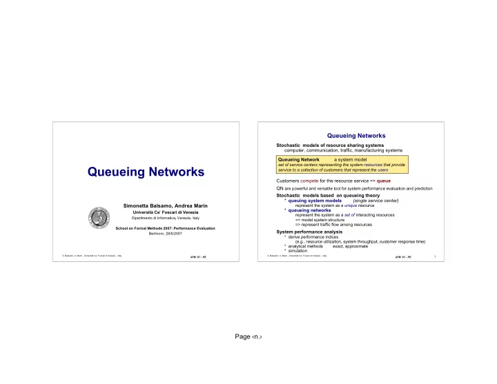
Queueing Networks Stochastic models of resource sharing systems computer, communication, traffic, manufacturing systems Queueing Network a system model set of service centers representing the system resources that provide Queueing Networks service to a collection of customers that represent the users Customers compete for the resource service => queue QN are powerful and versatile tool for system performance evaluation and prediction Stochastic models based on queueing theory * queuing system models (single service center) Simonetta Balsamo, Andrea Marin represent the system as a unique resource * queueing networks Università Ca’ Foscari di Venezia represent the system as a set of interacting resources Dipartimento di Informatica , Venezia, Italy => model system structure => represent traffic flow among resources School on Formal Methods 2007: Performance Evaluation System performance analysis Bertinoro, 28/5/2007 * derive performance indices (e.g., resource utilization, system throughput, customer response time ) * analytical methods exact, approximate * simulation S. Balsamo, A. Marin - Università Ca’ Foscari di Venezia - Italy 0 S. Balsamo, A. Marin - Università Ca’ Foscari di Venezia - Italy 1 SFM ‘07 - PE SFM ‘07 - PE Page ‹n.›
Outline Introduction: the queue Queueing systems I) - basic QN: Queueing Systems various hypotheses analysis to evaluate performance indices - Customers underlying stochastic Markov process arrive to the service center Queueing networks (QN) II) ask for resource service model definition possibly wait to be served => queueing discipline analysis to evaluate performance indices leave the service center types of customers: multi-chain, multi-class models types of QN Markovian QN service facility underlying stochastic Markov process arrivals departures Product-form QN III) have a simple closed form expression of the stationary state distribution BCMP theorem queue => efficient algorithms to evaluate average performance measures Solution algorithms for product-form QN Convolution, MVA, RECAL, … - under exponential and independence assumptions Properties of QN IV) one can define an associated stochastic continuous-time Markov process arrival theorem - exact aggregation - insensitivity to represent system behaviour Extensions and application examples special system features (e.g., state-dependent routing, negative customers, - performance indices are derived from the solution of the Markov process customers batch arrivals and departures and finite capacity queues) S. Balsamo, A. Marin - Università Ca’ Foscari di Venezia - Italy 2 S. Balsamo, A. Marin - Università Ca’ Foscari di Venezia - Italy 3 SFM ‘07 - PE SFM ‘07 - PE Page ‹n.›
Stochastic processes Markov processes Discrete-time Markov process Stochastic process: set of random variables {X n | n=1,2,...} {X(t) | t ∈ T} if the state at time n + 1 only depends on t he state probability at time n and defined over the same probability space indexed by the parameter t, called time is independent of the previous history each X(t) random variable Prob{X n+1 =j|X 0 =i 0 ;X 1 =i 1 ;...;X n =i n } =Prob{X n+1 =j|X n =i n } takes values in the set Γ called state space of the process ∀ n>0, ∀ j, i 0 , i 1 ,..., i n ∈ Γ Both T (time) and Γ (space) can be either discrete or continuous Continuos-time Markov process Continuous-time process if the time parameter t is continuous {X(t) | t ∈ T} if the time parameter t is discrete Discrete-time process Prob{X (t) =j|X(t 0 ) =i 0 ;X(t 1 )=i 1 ;...;X(t n )=i n } =Prob{X (t) =j| X(t n )=i n } {X n | n ∈ T } ∀ t 0 ,t 1 ,...,t n ,t : t 0 <t 1 <...<t n <t , ∀ n>0, ∀ j, i 0 , i 1 ,..., i n ∈ Γ Joint probability distribution function of the random variables X (t i ) Markov property Pr{X (t 1 ) ≤ x 1 ; X (t 2 ) ≤ x 2 ; . . . ; X (t n ) ≤ x n } The residence time of the process in each state is distributed according to geometric for discrete-time Markov processes for any set of times t i ∈ T , x i ∈ Γ , 1 ≤ i ≤ n, n ≥ 1 negative exponential distribution for continuous -time Markov processes Discrete-space Γ Markov processes are called Markov chain S. Balsamo, A. Marin - Università Ca’ Foscari di Venezia - Italy 4 S. Balsamo, A. Marin - Università Ca’ Foscari di Venezia - Italy 5 SFM ‘07 - PE SFM ‘07 - PE Page ‹n.›
Analysis of Markov processes Analysis of Markov processes Discrete-time Markov chain Continuous-time Markov chain {X n | n=1,2,...} {X(t) | t ∈ T} homogeneous if the one-step conditional probability is independent on time n homogeneous if the one-step conditional probability only depens on the p ij =Prob{X n+1 =j|X n =i} ∀ n>0, ∀ i,j ∈ Γ interval width P =[p ij ] state transition probability matrix p ij (s) =Prob{X(t+s) =j| X(t) =i} ∀ t>0, ∀ i,j ∈ Γ Q = lim s → 0 ( P (s) - I )/s If the stability conditions holds, we can compute the stationary state probability Q =[q ij ] matrix of state transition rates (infinitesimal generator) π =[ π 0 , π 1 , π 2 , …] π j =Pr{X=j} ∀ j ∈ Γ If the stability conditions holds, we compute the stationary state probability π =[ π 0 , π 1 , π 2 , …] For ergodic Markov chain (irreducible and with positively recurrent aperiodic states) π For ergodic Markov chain (irreducible and with positively recurrent aperiodic states) as can be computed as π Q = 0 with ∑ j π j =1 π = π P with ∑ j π j =1 system of global balance equations system of global balance equations S. Balsamo, A. Marin - Università Ca’ Foscari di Venezia - Italy 6 S. Balsamo, A. Marin - Università Ca’ Foscari di Venezia - Italy 7 SFM ‘07 - PE SFM ‘07 - PE Page ‹n.›
Birth-death Markov processes Birth-death Markov processes π =[ π 0 , π 1 , π 2 , …] Sufficient condition for stationary distribution State space Γ = N N T he only non-zero state transitions are those ∃ k 0 : ∀ k> k 0 λ k < µ k from any state i to states i − 1, i, i + 1, ∀ i ∈ Γ Matrix P (discrete-time) or Q (continuous-time) is tri-diagonal Special case : constant birth and death rates birth transition rate , i ≥ 0 λ i λ i = λ birth transition rate , i ≥ 0 continuos-time Markov chain µ i death transition rate, i ≥ 1 µ i = µ death transition rate, i ≥ 1 q i i+1 = λ i i ≥ 0 Let ρ = λ / µ q i i-1 = µ i i ≥ 1 If ρ <1 q i i = -( λ i + µ i ) i ≥ 1 q 00 = - λ 0 π 0 = [ ∑ k ρ k ] -1 = 1- ρ q i j = 0 |i-j|>1 π k = π 0 ( λ / µ ) k π k = (1- ρ ) ρ k k ≥ 0 Geometric distribution Closed-form expression Normalizing condition S. Balsamo, A. Marin - Università Ca’ Foscari di Venezia - Italy 8 S. Balsamo, A. Marin - Università Ca’ Foscari di Venezia - Italy 9 SFM ‘07 - PE SFM ‘07 - PE Page ‹n.›
Basic queueing systems Basic queueing systems n Single service center Single service center q w s 1 servente 1 server 2 … servente 2 server � m … queue coda t w t s servente m server popolazione population t q t r Δ : interarrival time w : number of customers in the queue t w : queue waiting time Customers resources offering a service s : number of customers in service t s : service time => resource contention n : number of customers in the system t r : response time S. Balsamo, A. Marin - Università Ca’ Foscari di Venezia - Italy 10 S. Balsamo, A. Marin - Università Ca’ Foscari di Venezia - Italy 11 SFM ‘07 - PE SFM ‘07 - PE Page ‹n.›
Definition of a queueing systems Analysis of a queueing systems • system analysis • The queueing system is described by Transient for a time interval, given the initial conditions * the arrival process Stationary in steady-state conditions, for stable systems * the service process • Analysis of the associated stochastic process that represents system * the number of servers and their service rate behavior * the queueing discipline process Markov stochastic process * the system or queue capacity birth and death processes * the population constraints • Evaluation of a set of performance indices of the queueing system • Kendall’s notation A/B/X/Y/Z * number of customers in the system n A interarrival time distribution ( Δ ) * number of customers in the queue w B service time distribution ( t s ) * response time t r X number of servers (m) * waiting time t w Y system capacity (in the queue and in service) * utilization U Z queueing discipline * throughput X A/B/X if Y = ∞ and Z = FCFS (default) random variables: evaluate probability distribution and/or the moments Examples: A,B : D deterministic (constant) M exponential (Markov) average performance indices Ek Erlang-k * average number of customers in the system N=E[n] G general * mean response time R=E[t r ] Examples of queueing systems: D/D/1, M/M/1, M/M/m (m>0), M/G/1, G/G/1 S. Balsamo, A. Marin - Università Ca’ Foscari di Venezia - Italy 12 S. Balsamo, A. Marin - Università Ca’ Foscari di Venezia - Italy 13 SFM ‘07 - PE SFM ‘07 - PE Page ‹n.›
Recommend
More recommend
Explore More Topics
Stay informed with curated content and fresh updates.
