Module 2 2.1 Transportation Planning Process The transportation - PDF document

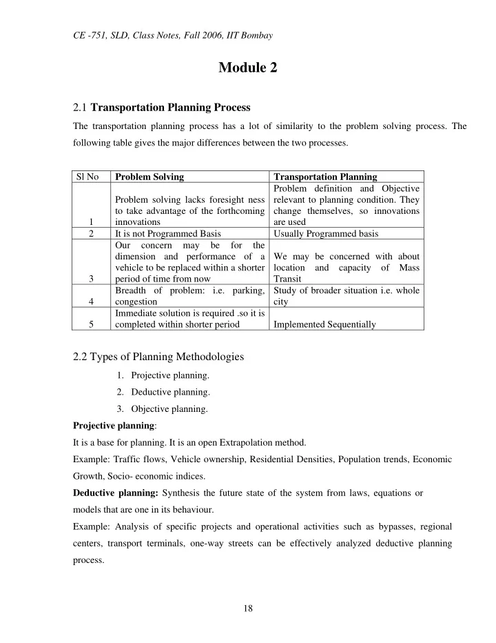
CE -751, SLD, Class Notes, Fall 2006, IIT Bombay Module 2 2.1 Transportation Planning Process The transportation planning process has a lot of similarity to the problem solving process. The following table gives the major differences between the two processes. Sl No Problem Solving Transportation Planning Problem definition and Objective Problem solving lacks foresight ness relevant to planning condition. They to take advantage of the forthcoming change themselves, so innovations 1 innovations are used 2 It is not Programmed Basis Usually Programmed basis Our concern may be for the dimension and performance of a We may be concerned with about vehicle to be replaced within a shorter location and capacity of Mass 3 period of time from now Transit Breadth of problem: i.e. parking, Study of broader situation i.e. whole 4 congestion city Immediate solution is required .so it is 5 completed within shorter period Implemented Sequentially 2.2 Types of Planning Methodologies 1. Projective planning. 2. Deductive planning. 3. Objective planning. Projective planning : It is a base for planning. It is an open Extrapolation method. Example: Traffic flows, Vehicle ownership, Residential Densities, Population trends, Economic Growth, Socio- economic indices. Deductive planning: Synthesis the future state of the system from laws, equations or models that are one in its behaviour. Example: Analysis of specific projects and operational activities such as bypasses, regional centers, transport terminals, one-way streets can be effectively analyzed deductive planning process. 18

CE -751, SLD, Class Notes, Fall 2006, IIT Bombay Objective planning: Planner sets some goals and with a certain objective and with constraints. It will be difficult to take into account the uncertainties. 2 4 3 1 Statement of Identification of objectives Modeling of Collection data on Transportation and constraints to be met by transportation present problems and proposed transportation systems and its transportation problem domain system Domain system and its domain 5 Calibration and use of models Projection of levels of Setting of levels of Prediction of levels of Regional land use transportation sub regional land use 13 development and other system variables development travel and affecting variables other affected variables Operation and 6 8 Maintenance of system 10 Evaluation of Generation and Specification of 11 7 9 performance and resetting of details of selected Implementation of decision among transportation transportation system changes alternative systems system variables systems 12 Total Transportation planning process 19

CE -751, SLD, Class Notes, Fall 2006, IIT Bombay Deductive Planning Process 2.3 Travel demand modelling: There are four steps of travel demand modelling. They are 1. Trip generation 2. Model split 3. Trip Distribution 4. Trip assignment 20

CE -751, SLD, Class Notes, Fall 2006, IIT Bombay Steps of Travel Demand Modelling 2.3.1 Trip-Generation Analysis : -Two types of trip-generation analysis are carried out and these are trip production and trip attraction. Trip Production : -is reserved for trips generated by residential zones where these trips may be trip origins and destinations. Trip Attraction : -is used to describe trips generated by activities at the non-home end of a home-based trip such as employment, retail service, and so on. 21

CE -751, SLD, Class Notes, Fall 2006, IIT Bombay The first activity in travel-demand forecasting is to identify the various trip types important to a particular transport-planning study. The trip types studied in a particular area depend on the types of transport-planning issues to be resolved. The first level of trip classification used normally is a broad grouping into home-based and non-home-based trips. Home-based Trips : - are those trips that have one trip end at a household. Examples journey to work, shop, school etc. Non-home-based trips : -are trips between work and shop and business trips between two places of employment. Trip classification that have been used in the major transport-planning studies for home-based trips are: a. Work trips b. School trips c. Shopping trips d. Personnel business trips, and e. Social-recreational trips Factors influencing Trip Production Households may be characterized in many ways, but a large number of trip-production studies have shown that the following variables are the most important characteristics with respect to the major trip trips such as work and shopping trips: 1. The number of workers in a household, and 2. The household income or some proxy of income, such as the number of cars per household. Factors Influencing Trip Attraction Depending on the floor areas, the trip attraction can be determined from retail floor area, service and office floor area and manufacturing and wholesaling floor area. Multiple Regression Analysis The majority of trip-generation studies performed have used multiple regression analysis to develop the prediction equations for the trips generated by various types of land use. 22

CE -751, SLD, Class Notes, Fall 2006, IIT Bombay Most of these regression equations have been developed using a stepwise regression analysis computer program. Stepwise regression –analysis programs allow the analyst to develop and test a large number of potential regression equations using various combinations and transformations of both the dependent and independent variables. The planner may then select the most appropriate prediction equation using certain statistical criteria. In formulating and testing various regression equations, the analyst must have a thorough understanding of the theoretical basis of the regression analysis. Review of Regression Analysis Concept Some of the fundamental of regression analysis: - The principal assumptions of regression analysis are: 1. The variance of the Y values about the regression line must be the same for all magnitudes of the independent variables. 2. The deviations of the Y values about the regression line must be independent of each other and normally distributed. 3. The X values are measured without error 4. The regression of the dependent variable Y on the independent variable X is linear. Assume that observation of the magnitude of a dependent variable Y have been obtained for N magnitudes of an independent variable X and that on an equation of the form = + Y e a bX is to be fitted to the data where Y is an estimated magnitude rather than an e observed value Y . From the least-squares criterion, the magnitude of the parameters a and b may be estimated. ∑ xy = b ∑ 2 x = − a Y b X where = − = − x X X and y Y Y 23

CE -751, SLD, Class Notes, Fall 2006, IIT Bombay X , Y =the means of the X and Y observations respectively. ∑ ∑ ∑ = + 2 2 2 y y y d e Where ∑ 2 y = total sum of the squares of the deviations of the Y observations about the mean value ∑ 2 y =the sum of the squares of the deviations of the Y observations from the d regression line. ∑ 2 y =the sum of the squares of the deviations of the estimated Y magnitude about e e the mean value. The ratio of the sum of the squares explained by the regression to the total sum of squares is known as the coefficient of determination and denoted by r 2 . ∑ 2 y 2 ≤ e = ≤ r 2 r 0 1 ∑ 2 y • if 2 =1 implies no variation remaining that is unexplained by the independent r variable used in the regression. • If 2 r = 0 implies the independent variable used would not explain any of the observed variation in the dependent variable. The square root of the coefficient of determination is termed as the correlation coefficient. A second useful measure of the validity of a regression line is the standard error of the estimate, which is estimated from: ∑ 2 y = d s − e ( N 2 ) 24

CE -751, SLD, Class Notes, Fall 2006, IIT Bombay where is the degree of freedom associated with the sum of squares ∑ − 2 ( N 2 ) y d The regression coefficient b is the statistical estimate and is therefore subject to error. s b = e s N s X where s is the standard deviation of the independent variable. X Statements about the confidence that might be placed in an estimated coefficient is given by: t = regression coefficient standard error of the regression coefficient Partial or Multiple Regression Equation It has equation of the form: = + + + + Y a b X b X ... b X e 1 1 2 2 p p where there are p independent variables and the regression coefficients b , b ,…, b 1 2 p are referred to as partial regression coefficients . 2 is given by: 2 The coefficient of multiple determinations, R ∑ − 2 R = ∑ ( Y e Y ) 2 − 2 ( Y Y ) 2 where R is known as the multiple correlation coefficients. ∑ 2 y = e s − + e [ N ( P 1 )] 25