Models of ice sheet dynamics and meltwater lubrication Ian Hewitt, - PowerPoint PPT Presentation

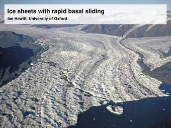
Models of ice sheet dynamics and meltwater lubrication Ian Hewitt, University of Oxford Thanks to: Christian Schoof, Mauro Werder, Gwenn Flowers, John Fell Fund, ERC

Antarctica B B ' West Antarctica 4,000 Ellsworth Ice Elevation (m) Mountains Land 2,000 Ocean Ronne Ice Shelf Ross Ice Shelf (MSL) 0 -2,000 0°E C Vertical exaggeration x80 Bentley Subglacial Trench 30°E 30°W B Ice velocity 60°W 60°W 60°W 60°E 60°E 60°E (m year –1 ) 1,000 100 90°W 90°E 90°E 90°E 10 S ° 0 8 S <1.5 ° 0 7 120°E 120°E 120°E 120°W B ' 150°E 150°E 150°E 150°W C ' 180°E East Antarctica C C ' 4,000 Elevation (m) Gamburtsev Subglacial Vostok Subglacial Mountains 2,000 Highlands Gunnerus Bank (MSL) 0 -2,000 Vertical exaggeration x80 Aurora Vincennes Astrolabe Subglacial Basin Subglacial Basin Subglacial Basin

Ice sheets in climate models Most climate models have a static ice sheet The ice sheet stores and releases water according to surface energy balance Some interesting feedbacks are (at least potentially!) not captured

Models of ice sheet dynamics Stokes flow r · u = 0 r · u ∂τ ij � ∂ p = � ρ g i ✓ ∂ x j ∂ x i q D ij = 1 ✓ ∂ u i ◆ + ∂ u j q Rheology τ ij = A − 1 /n D 1 /n − 1 D ij 1 D = 2 D ij D ij 2 ∂ x j ∂ x i ⇡ A = A ( T ) n ⇡ 3 Boundary conditions surface � pn i + τ ij n j = 0 ( δ ij � n i n j ) τ jk n k = f ( U b )( δ ij � n i n j ) u i ◆ bed U b ∂ s ∂ t + u ∂ s ∂ x + v ∂ s surface ∂ y = w + a � pn i + τ ij n j = 0 z = s ◆ u ∂ b ∂ x + v ∂ b bed ∂ y = w − m Ice z = b z τ b = f ( U b ) u b Bedrock x U b

Reduced models (depth-integrated) Shallow ice approximation Z z = s ∂ s � ( s � b ) n +2 | r s | n − 1 r s � ∂ t � r · = a � m z = b Shallow stream approximation z = s � � z = b ∂ H ∂ t + r · ( H u ) = a � m  ✓ ◆�  ✓ ∂ u ◆� f ( U b ) u = � ρ gH ∂ s ∂ x + ∂ 4 ∂ u ∂ x + 2 ∂ v + ∂ ∂ y + ∂ v η H η H U b ∂ x ∂ y ∂ y ∂ x  ✓ ∂ u ◆�  ✓ ◆� f ( U b ) v = � ρ gH ∂ s ∂ y + ∂ ∂ y + ∂ v + ∂ 2 ∂ u ∂ x + 4 ∂ v η H η H U b ∂ x ∂ x ∂ y ∂ y

Inverse methods

Inversion for basal slipperiness (frozen-time problem) Stokes flow r · u = 0 r · u ∂τ ij � ∂ p = � ρ g i ∂ x j ∂ x i Assume a linear friction law f ( U b ) = β U b Basal boundary condition τ b = β ( x ) u b Forward problem : given geometry, temperature & basal slipperiness, determine ice velocity Inverse problem : use observed ice velocity to infer basal slipperiness J ( β ) = 1 Z | u − u obs | 2 d V + R ( β ) 2

Surface velocity Inversion for basal slipperiness Observations Model Inferred basal slipperiness Isaac et al 2015

Inversion for bed topography (assumes steady state) c d 70 ° W 60 ° W 80 ° N 30 km 50 km 75 ° N b e 70 ° N 20 km 30 km a f 65 ° N 300 km W ° 0 50 ° W 40 ° W 3 6 0 ° N 20 km 20 km − 500 0 500 1,000 1,500 2,000 Morlighem et al 2014 Bed elevation (m)

Future Assimilate time-dependent observations Make use of more observations - eg. internal radar layers Duncan Young / UTIG

Sliding

Microscopic view of a ‘hard’ bed τ b β u b A film of water exists between ice and the underlying bedrock, allowing slip Resistance comes from the roughness of the bedrock τ b = β u b ‘Cavitation’ occurs in the lee of bumps

Nye’s sliding theory � Newtonian ice Stokes flow � 4 ψ = 0 ⇤ ν � 1 � 2 T = 0 Heat equation ⇤ � � ρ i L ⇤ ∞ ˆ ⇥ 1 / 2 k 2 Z b ( k ) k 3 Take Fourier transform k ∗ = τ b = η i U b ∗ d k k 2 + k 2 4 kC η π 0 ∗ � ⇥ � ⌅ M � � 1 Z b ( x ) e ikx d x ˆ � � Fourier transform of bed profile, i.e. power spectrum Z b ( k ) = lim � � M M →∞ � � − M Theory can be extended to account for cavitation Riemann-Hilbert problem � ⌅ � � � →∞ � Stokes flow � 4 ψ = 0 − ⇥ U b ⇤ τ b = Nf ⇤ N ν � 1 ⇥ ⇤ �⌅ Nye 1969, Fowler 1986, Schoof 2005

Sliding laws τ b τ b β u b � ⇥ Hard bedrock τ b = RU 1 /m b ⇥ U b τ b β u b Cavities τ b /N τ b = CN q U p � ⇥ b ⇥ 1 /n � U b ⇧ b = µN U b + ⇤ AN n ⇥ U b /N n τ b β u b Soft sediments τ b /N (plastic) τ b = µN � U b /N n

Subglacial water

A distributed drainage model Ice surface ‘Water table’ z = s h Basal water z = b ∂ h ∂ t + r · q = m + r q = � K ( h ) r φ φ = ρ gb + p w φ ⇡ ρ gs + ( ρ w � ρ ) gb

10 m

Turbulent dissipation causes channelisation Analogues Chemical erosion (eg limestone caves) h Mechanical erosion S ‘Wormholing’

Cordillera Blanca, Peru

Subglacial conduits z = s ⇡ � z = b φ = ρ gs + ( ρ w � ρ ) gb � N ⇤ ⇤ ⇤ ⇤ ⇤ ⇤ ⇤ ⇤ Creep − 1 / 2 ∂φ ⇤ ⇤ ∂φ Flux Q = − K c S α ⇤ ⇤ ⇤ ⇤ ∂ s ∂ s ⇤ ⇤ Melting Cross-sectional area evolution M − 2 A ∂ S ∂ t = ρ w n n S | N | n − 1 N ρ i ⇤ ⇤ ⇤ ⇤ 1 ⇤ Q ∂φ Melting ⇤ ⇤ M = ⇤ ⇤ ρ w L ∂ s ⇤ Mass conservation ⇤ ⇤ ∂ S ∂ t + ∂ Q Energy ∂ s = M + q in ⇠ gH ⇠ c p T H ⇡ 1 km T ≈ 2 . 5 K ⇠ ⇡ gH ⇠ φ L φ ⇡ 0 . 03 Röthlisberger 1972, Nye 1976

Subglacial conduits Creep ∂ S ∂ t = C 1 S α Ψ 3 / 2 � C 2 SN n α > 1 Melting ∂ S ∂ t C 2 S Unstable equilibrium Q Mass conservation prevents unbounded growth ... but neighbouring channels compete with one other