Modelling the Business Cycle Siem Jan Koopman - PowerPoint PPT Presentation
Modelling the Business Cycle Siem Jan Koopman s.j.koopman@feweb.vu.nl Vrije Universiteit Amsterdam Tinbergen Institute Modelling the Business Cycle p. 1 Eurozone GDP Data 14.25 14.20 14.15 14.10 14.05 14.00 13.95 13.90 1985 1990
Modelling the Business Cycle Siem Jan Koopman s.j.koopman@feweb.vu.nl Vrije Universiteit Amsterdam Tinbergen Institute Modelling the Business Cycle – p. 1
Eurozone GDP Data 14.25 14.20 14.15 14.10 14.05 14.00 13.95 13.90 1985 1990 1995 2000 Modelling the Business Cycle – p. 2
Topics in Business Cycle Analysis • dating of business cycles (Markov-switching models) • prinicipal components analysis (Stock and Watson, Forni, Hallin, Lippi and Reichlin) • convergence and synchronisation (economic theory, empirical studies) • asymmetry and nonlinearities (econometrics) • coincident and leading indicators (economics) Aim is to detect business cycle and growth • Detrending methods (Hodrick-Prescott); • Bandpass filtering methods (Baxter-King, Christiano-Fitzgerald); • Model-based, univariate (Beveridge-Nelson, Clark, Harvey-Jaeger); • Model-based, multivariate, common cycles (VAR model, UC model). Modelling the Business Cycle – p. 3
Different Univariate Trend-Cycle Decompositions 0.02 0.01 14.2 0.00 14.0 −0.01 HP trend HP cycle 1985 1990 1995 2000 1985 1990 1995 2000 14.3 0.01 14.2 14.1 0.00 14.0 STAMP trend 13.9 STAMP cycle −0.01 1985 1990 1995 2000 1985 1990 1995 2000 0.01 14.2 0.00 14.0 −0.01 AKR trend AKR cycle 1985 1990 1995 2000 1985 1990 1995 2000 Modelling the Business Cycle – p. 4
Univariate UC Trend-Cycle Decomposition y t = µ t + ψ t + ε t • Trend µ t : ∆ d µ t = η t ; • Irregular ε t : White Noise; • Cycle ψ t : AR(2) with complex roots as in Clark (87) or with stochastic trigonometric functions as in Harvey (85,89); Trigonometric specification: � � � � � � � � ψ t +1 cos λ sin λ ψ t κ t = φ + , ψ + ψ + κ + − sin λ cos λ t +1 t t ∼ NID (0 , σ 2 κ t , κ + κ ) . t Signal extraction is about (locally) weighting observations. Kalman filter gives the optimal weights for the given models. Modelling the Business Cycle – p. 5
Weights and Gain Functions of Components 14.3 0.02 14.2 14.1 0.00 14.0 13.9 −0.02 1985 1990 1995 2000 1985 1990 1995 2000 0.2 0.5 0.1 0.0 0.0 −20 −10 0 10 20 −20 −10 0 10 20 1.0 1.0 0.5 0.5 0.0 0.2 0.4 0.6 0.8 1.0 0.0 0.2 0.4 0.6 0.8 1.0 Modelling the Business Cycle – p. 6
Band-pass Properties "Band-pass" refers to frequency domain properties of polynomial lag functions of time series (filters). In business cycle analysis, one is interested in filters for trend and cycles such that trend only captures the low-frequencies, cycle the mid-frequencies and irregular the high frequencies. 1.0 0.5 TREND 0.0 0.1 0.2 0.3 0.4 0.5 0.6 0.7 0.8 0.9 1.0 1.0 0.5 CYCLE 0.0 0.1 0.2 0.3 0.4 0.5 0.6 0.7 0.8 0.9 1.0 1.0 0.5 IRREGULAR 0.0 0.1 0.2 0.3 0.4 0.5 0.6 0.7 0.8 0.9 1.0 Modelling the Business Cycle – p. 7
Butterworth Filters for Trend Butterworth trend filters can be considered; they have a model-based representation and can be put in state space framework; see Gomez (2001). The m -th order stochastic trend is µ t = µ ( m ) where t ∆ m µ ( m ) ζ t ∼ NID (0 , σ 2 t +1 = ζ t , ζ ) , or µ ( j ) t +1 = µ ( j ) + µ ( j − 1) “ j = m, m − 1 , . . . , 1 , , t t with µ (0) = η t as before. t For m = 2 we have IRW with β t = µ (1) t . Higher value for m gives low-pass gain function with sharper cut-off downwards at certain low frequency point. Modelling the Business Cycle – p. 8
Generalised Cycle Same principles can be applied to the cycle. The generalised k th order cycle is given by ψ t = ψ ( k ) , where t � ψ ( j ) � � � � ψ ( j ) � � ψ ( j − 1) � cos λ sin λ t +1 t t = φ + , ψ +( j ) ψ +( j ) ψ +( j − 1) − sin λ cos λ t +1 t t j = 1 , . . . , k, with � � � � ψ (0) κ t t = . ψ +(0) κ + t ‘ m t Higher orders ensure smoother transitions. Further details: Trimbur (2002), Harvey & Trimbur (2003). Modelling the Business Cycle – p. 9
Weights and Gain Functions of Components 14.3 0.02 14.2 14.1 0.00 14.0 13.9 −0.02 1985 1990 1995 2000 1985 1990 1995 2000 0.2 0.5 0.1 0.0 0.0 −20 −10 0 10 20 −20 −10 0 10 20 1.0 1.0 0.5 0.5 0.0 0.2 0.4 0.6 0.8 1.0 0.0 0.2 0.4 0.6 0.8 1.0 Modelling the Business Cycle – p. 10
Measuring a common cycle from a multiple time series • Analysis is based on a multivariate model • Data-set includes series that are leading, lagging GDP • We prefer not to choose leads & lags a-priori • Common cycle will be allowed to shift for individual time series using techniques developed by Rünstler (2002). 0.2 0.0 −0.2 estimated cycles gdp (red) versus cons confidence (blue) −0.4 1980 1985 1990 1995 0.2 0.0 −0.2 estimated cycles gdp (red) versus shifted cons confidence (blue) −0.4 1980 1985 1990 1995 Modelling the Business Cycle – p. 11
Shifted cycles In standard case, cycle ψ t is generated by � � � � � � � � cos λ sin λ ψ t +1 ψ t κ t = φ + ψ + ψ + κ + − sin λ cos λ t +1 t t The cycle cos( ξλ ) ψ t + sin( ξλ ) ψ + t , is shifted ξ time periods to the right (when ξ > 0 ) or to the left (when ξ < 0 ). Here, − 1 2 π < ξ 0 λ < 1 2 π (shift is wrt ψ t ) More details in Rünstler (2002) for idea of shifting cycles in multivariate unobserved components time series model of Harvey and Koopman (1997). Modelling the Business Cycle – p. 12
The basic multivariate model Panel of N economic time series, y it , ε it ∼ NID (0 , σ 2 y it = µ it + δ i ψ t + ε it , i,ε ) The time series have mixed frequencies (quarterly and monthly) Final model: shifted cycles in model via the formulation � � y it = µ ( k ) cos( ξ i λ ) ψ ( m ) + sin( ξ i λ ) ψ +( m ) it + δ i + ε it , t t with • generalised individual trend µ ( k ) it , • generalised common cycle ψ ( m ) (with associated variable ψ +( m ) ) t t • irregular ε it . Modelling the Business Cycle – p. 13
Business cycle Stock and Watson (1999): “ . . . fluctuations in aggregate output are at the core of the business cycle so the cyclical component of real GDP is a useful proxy for the overall business cycle . . . ” We therefore impose a unit common cycle loading and zero phase shift for Euro area real GDP . Time series 1986 – 2002 * quarterly GDP * industrial production * unemployment (countercyclical, lagging) * industrial confidence * construction confidence * retail trade confidence * consumer confidence * retail sales * interest rate spread (leading) Modelling the Business Cycle – p. 14
Eurozone Economic Indicators 14.30 GDP Retail sales IPI unemployment Interest rate spread Industrial confidence indicator Construction confidence indicator Retail trade confidence indicator 14.25 Consumer confidence indicator 14.20 14.15 14.10 14.05 14.00 13.95 13.90 1990 1995 2000 Modelling the Business Cycle – p. 15
Details of model, estimation • we have set m = 2 and k = 6 for generalised components • leads to estimated trend/cycle estimates with band-pass properties, Baxter and King (1999). • frequency cycle is fixed at λ = 0 . 06545 ( 96 months, 8 years), see Stock and Watson (1999) for the U.S. and ECB (2001) for the Euro area • shifts ξ i are estimated • number of parameters for each equation is four ( σ 2 i,ζ , δ i , ξ i , σ 2 i,ε ) and for the common cycle is two ( φ and σ 2 κ ) • total number is 4 N = 4 × 9 = 36 Modelling the Business Cycle – p. 16
Decomposition of real GDP 14.2 0.003 14.1 0.002 14.0 0.001 GDP Euro Area Trend slope 13.9 1990 1995 2000 1990 1995 2000 0.01 0.0050 0.0025 0.00 0.0000 −0.0025 −0.01 −0.0050 irregular Cycle 1990 1995 2000 1990 1995 2000 Modelling the Business Cycle – p. 17
The business cycle coincident indicator Noteworthy features: • GDP is quarterly, estimated components are monthly • Euro area potential growth has declined after major recession of 1993 (before, growth was around 3 . 7% in annualised terms, after it was 2 . 4% , falls within the 2 . 0 − 2 . 5 underlying the ECB monetary policy) • GDP cycle in line with common wisdom regarding Euro area business cycle, ECB (2002) • business cycle tracks the turning points well • historical minimum value is observed in Aug 1993, falls in most severe recession period of Euro area • maximum value is in Jan 2001 Modelling the Business Cycle – p. 18
The business cycle coincident indicator Selected estimation results R 2 series load shift d gdp −− −− 0 . 31 1 . 18 6 . 85 0 . 67 indutrial prod − 0 . 42 − 15 . 9 Unemployment 0 . 78 industriual c 2 . 46 7 . 84 0 . 47 construction c 0 . 77 1 . 86 0 . 51 0 . 26 − 0 . 22 0 . 67 retail sales c consumer c 1 . 12 3 . 76 0 . 33 − 4 . 70 retail sales 0 . 11 0 . 86 int rate spr 0 . 57 16 . 8 0 . 22 Modelling the Business Cycle – p. 19
Coincident indicator for Euro area business cycle 0.010 0.005 0.000 −0.005 −0.010 −0.015 1990 1995 2000 Modelling the Business Cycle – p. 20
Recommend
More recommend
Explore More Topics
Stay informed with curated content and fresh updates.

