Modeling Cloud Reflectance Fields Using Condi4onal Genera4ve - PowerPoint PPT Presentation
Modeling Cloud Reflectance Fields Using Condi4onal Genera4ve Adversarial Networks Victor Schmidt, Mustafa Alghali, Kris Sankaran, Tianle Yuan, Yoshua Bengio. ICLR-CCAI 2020 All code and hyperparameters may be found at
Modeling Cloud Reflectance Fields Using Condi4onal Genera4ve Adversarial Networks Victor Schmidt, Mustafa Alghali, Kris Sankaran, Tianle Yuan, Yoshua Bengio. ICLR-CCAI 2020 All code and hyperparameters may be found at https://github.com/krisrs1128/clouds_dist
(1) Mo4va4on
Global Climate Models (GCMs) • GCMs had huge success in simula1ng the earth’s weather, energy balance, and predic1ng possible changes in climate [1] including but not limited to: [Henderson and Sellers, 1985] changes in precipita-on* increases in temperatures** accelera-on in glacial mel-ng*** • One of the key physical principles these models rely on is the Earth’s energy balance [2] ** Future impacts of climate change on forests * USGS water science school *** scien2ficamerican.com
Clouds modeling and earth’s energy balance • Clouds play an important role in earth’s energy balance as they both reflect energy coming to the Earth and the infrared radiations it emits .[3] • However, as physical processes at play in cloud composition and evolution typically range from 10 -6 to 10 6 m, direct simulation of their behavior can consume up to 20% of a GCM’s computations .[4, 5, 6] [ Schneider, Stephen H. "Climate modeling." Scientific American 256.5 (1987): 72-T9] Modeling clouds accurately using GCMs is challenging and expensive. •
Cloud modeling computa0onal complexity Various efforts have tried to address this challenge such as: • Incorporate more domain knowledge • super-parameteriza1on (modeling sub-grids) ✔ Machine learning (model sub-grid using meteorological variables) [7, 8, 9, 10]
(2) Approach
Narrowing down the clouds modeling challenge 🎰 In our approach we propose modeling Cloud Reflectance Fields (CRFs) using conditional Generative Adversarial Networks (GANs) • We suggest using the generated CRFs as a proxy from which we can extract important cloud parameters such as optical depth and integrate these parameters into GCMs (it is not an alternative to GCMs) • We believe our approach is a step towards building a data-driven framework that can reduce the computational complexity in traditional cloud modeling techniques.
Approach: overview • We use GAN to generate cloud reflectance fields condi1oned on meteorological variables, taking the climate chao1c nature into considera1on. Extract important cloud parameters such as Condi-onal op1cal depth GAN • • • Meteorological variables Cloud reflectance fields
Approach: Data • Training data: 3100 aligned sample pairs X = {m i , r i } • Independent variable (m i ) 🌢 : is a 44 × 256 × 256 matrix, represen1ng 42 measurements from NASA’s MERRA-2 [19] along with longitude and la1tude to account for the Earth’s movement rela1ve to the satellite. • Dependent variable (r i ) 🌐 : is a 3 × 256 × 256 matrix represen1ng each loca1on’s reflectance at RGB wavelengths (680, 550 and 450 nm) as measured by the Aqua dataset [20] .
(3) Methodology
Architecture: Generator • U-Net generator [11] • Skip connec1ons help localiza1on • reduce the need for larger training set Checkerboard ar2facts [12] ∼ 1.4 million parameters • Upsampling followed by a convolu1on instead of transposed • convolu1on
Architecture: Discriminator • Multi-scale discriminator [13] • Better guide for the generator both in the scale of global context and finer details in the image. Global scale e.g. earth Medium scale e.g. Con2nents and oceans disk {Real, Generated} Finer structure e.g. cloud shapes and edges ∼ 8.3 million parameters
Training objec0ve Total GAN loss Less blurry output than L 2 loss Least square loss (LSGAN) [14] Hinge loss [15]
Challenges: Op=miza=on Adam/SGD • Extra_SGD [17] • ✔ Extra-Adam [17] see code at h;ps://github.com/GauthierGidel/VariaAonal-Inequality-GAN
Challenges: Regression vs. hallucinated features
Challenges: Sharpness of generated images Prematurely saturated learning (Nash equilibrium) [18] • Carefully choose the discriminator learning rate! 🎰 •
(4) Results
Visual Analysis • Generated images look difficult to dis1nguish from true samples with average L 2 distance ~ 0.027 on valida1on set. Generated Real Generated Real (left) (right) (leE) (right) • Valida1on set is set to 5 samples that are selected manually to capture different regions of the rota1ng earth. • Generate 15 samples in total: 3 for each valida1on sample. Model inference on never seen examples
Visual Analysis: Quan=fying ensemble diversity • For each ensemble genera1on we calculate: • Pixel-wise mean • Standard devia1on • Inter-quar1le range (IQR) Ensemble generation conditioned on the same input • Tradeoff (genera1on quality ↔ genera1on diversity)
Spectral Analysis • Visual inspec1on is an expensive, cumbersome, and subjec1ve measure! • Spectral analysis: ✔ Similar DFT distribu1ons but there is s1ll room for improvement ✔ Very small average L2 loss of 0.006 per frequency component. Frequency components Image Frequency distribu-on magnitude Real Generate d
What’s next? • Blurriness and small size checkerboard ar1facts: ❑ More training samples ❑ More hyperparameter tuning → avoid prematurely saturated learning. ❑ Longer training
What’s next? Exploit temporal structure 🕔 : ● ○ Add date and 1me as extra labels to the input variable. ○ Using nested temporal cross valida1on to predict possible changes in cloud distribu1on over 1me. Increase the diversity in the generated ensembles. 🎩 ● ○ Incorporate input noise channels as an extra source of stochas1city ○ Address mode collapse by using decaying λ2 𝜇 ! =exp(-t) epochs ● Modeling low clouds a key source of uncertainty in our ability to project future climate changes [21]
Appendix A: Data
Appendix B: Data processing • Sensor noise Winsorization → clip CRFs to the 95 th percentile. • Standardization • Avoid introducing unnecessary bias in the data distribution by the values outside the earth disk o Reduce them by zooming (crop & then resize using 2D nearest neighbor) o Replace other remaining values with -3 (mean - 3x standard deviation) • Use running statistics → mitigate shortage of GPU memory budget • Use 12 data loader workers → speed up the data loading process 6x
Appendix C: Hyperparameters
References: [1] Thomas F Stocker, Dahe Qin, Gian-Kasper Pla[ner, Melinda Tignor, Simon K Allen, Judith Boschung, Alexander Nauels, Yu Xia, Vincent Bex, Pauline M Midgley, et al. Climate change 2013: The physical science basis. Contribu)on of working group I to the fi4h assessment report of the intergovernmental panel on climate change , 1535, 2013. [2] Gerald R North, Robert F Cahalan, and James A Coakley Jr. Energy balance climate models. Reviews of Geophysics , 19(1):91–121, 1981. [3] VLRD Ramanathan, RD Cess, EF Harrison, P Minnis, BR Barkstrom, E Ahmad, and D Hart- mann. Cloud-radia-ve forcing and climate: Results from the earth radia-on budget experiment. Science , 243(4887):57–63, 1989. [4] Akio Arakawa. The cumulus parameteriza-on problem: Past, present, and future. Journal of Climate , 17(13):2493–2525, 2004. [5] Christopher S Bretherton. Insights into low-la-tude cloud feedbacks from high-resolu-on models. Philosophical Transac)ons of the Royal Society A: Mathema)cal, Physical and Engineering Sciences , 373(2054):20140415, 2015. [6] Tapio Schneider, João Teixeira, Christopher S Bretherton, Florent Brient, Kyle G Pressel, Christoph Schär, and A Pier Siebesma. Climate goals and compu-ng the future of clouds. Nature Climate Change , 7(1):3–5, 2017.
References: [7] Noah D Brenowitz and Christopher S Bretherton. Prognos-c valida-on of a neural network unified physics parameteriza-on. Geophysical Research LeJers , 45(12):6289–6298, 2018. [8] Stephan Rasp, Michael S Pritchard, and Pierre Gen-ne. Deep learning to represent subgrid processes in climate models. Proceedings of the Na)onal Academy of Sciences , 115(39): 9684–9689, 2018. [9] Paul A O’Gorman and John G Dwyer: Using machine learning to parameterize moist convec-on: Poten-al for modeling of climate, climate change, and extreme events. Journal of Advances in Modeling Earth Systems , 10(10):2548–2563, 2018. [10] T. Yuan, H. Song, D. Hall, V. Schmidt, K. Sankaran, and Y. Bengio. Ar-ficial intelligence based cloud distributor (ai-cd): probing clouds with genera-ve adversarial networks. AGU Fall Mee)ng 2019 , 2019. [11] Olaf Ronneberger, Philipp Fischer, and Thomas Brox. U-net: Convolu-onal networks for biomedical image segmenta-on. In Interna)onal Conference on Medical image compu)ng and computer-assisted interven)on , pp. 234–241. Springer, 2015. [12] Augustus Odena, Vincent Dumoulin, and Chris Olah. Deconvolu-on and checkerboard ar-facts. Dis)ll , 1(10):e3, 2016.
Recommend
More recommend
Explore More Topics
Stay informed with curated content and fresh updates.
