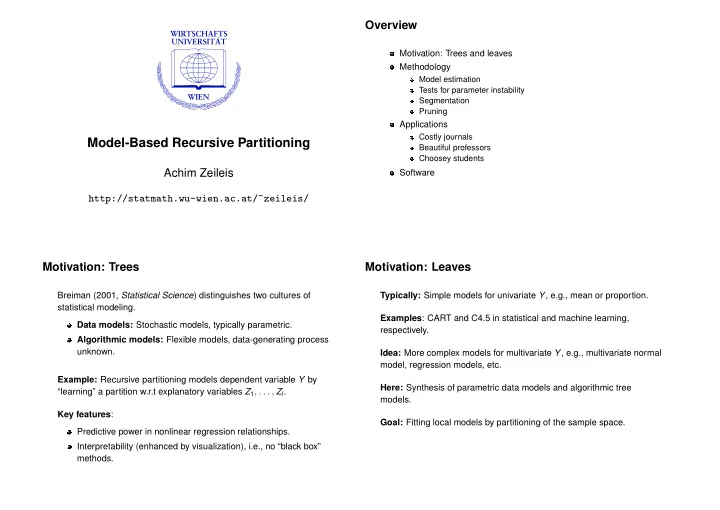
Model-Based Recursive Partitioning Beautiful professors Choosey - PowerPoint PPT Presentation

Overview Motivation: Trees and leaves Methodology Model estimation Tests for parameter instability Segmentation Pruning Applications Costly journals Model-Based Recursive Partitioning Beautiful professors Choosey students Achim Zeileis Software http://statmath.wu-wien.ac.at/~zeileis/ Motivation: Trees Motivation: Leaves Breiman (2001, Statistical Science ) distinguishes two cultures of Typically: Simple models for univariate Y , e.g., mean or proportion. statistical modeling. Examples : CART and C4.5 in statistical and machine learning, Data models: Stochastic models, typically parametric. respectively. Algorithmic models: Flexible models, data-generating process unknown. Idea: More complex models for multivariate Y , e.g., multivariate normal model, regression models, etc. Example: Recursive partitioning models dependent variable Y by Here: Synthesis of parametric data models and algorithmic tree “learning” a partition w.r.t explanatory variables Z 1 , . . . , Z l . models. Key features : Goal: Fitting local models by partitioning of the sample space. Predictive power in nonlinear regression relationships. Interpretability (enhanced by visualization), i.e., no “black box” methods.

Recursive partitioning 1. Model estimation Models: M ( Y , θ ) with (potentially) multivariate observations Y ∈ Y Base algorithm : and k -dimensional parameter vector θ ∈ Θ . Fit model for Y . 1 Assess association of Y and each Z j . Parameter estimation: � 2 θ by optimization of objective function Ψ( Y , θ ) Split sample along the Z j ∗ with strongest association: Choose for n observations Y i ( i = 1 , . . . , n ): 3 breakpoint with highest improvement of the model fit. n � Repeat steps 1–3 recursively in the sub-samples until some � 4 θ = Ψ( Y i , θ ) . argmin stopping criterion is met. θ ∈ Θ i = 1 Special cases: Maximum likelihood (ML), weighted and ordinary least Here: Segmentation (3) of parametric models (1) with additive objective squares (OLS and WLS), quasi-ML, and other M-estimators. function using parameter instability tests (2) and associated statistical significance (4). Central limit theorem: If there is a true parameter θ 0 and given certain weak regularity conditions, ˆ θ is asymptotically normal with mean θ 0 and sandwich-type covariance. 1. Model estimation 2. Tests for parameter instability Estimating function: � Generalized M-fluctuation tests capture instabilities in � θ can also be defined in terms of θ for an ordering w.r.t Z j . n � ψ ( Y i , � θ ) = 0 , Basis: Empirical fluctuation process of cumulative deviations w.r.t. to i = 1 an ordering σ ( Z ij ) . where ψ ( Y , θ ) = ∂ Ψ( Y , θ ) /∂θ . ⌊ nt ⌋ � W j ( t , � B − 1 / 2 n − 1 / 2 � ψ ( Y σ ( Z ij ) , � θ ) = θ ) ( 0 ≤ t ≤ 1 ) Idea: In many situations, a single global model M ( Y , θ ) that fits all i = 1 n observations cannot be found. But it might be possible to find a partition w.r.t. the variables Z = ( Z 1 , . . . , Z l ) so that a well-fitting model Functional central limit theorem: Under parameter stability can be found locally in each cell of the partition. → W 0 ( · ) , where W 0 is a k -dimensional Brownian bridge. d W j ( · ) − Tool: Assess parameter instability w.r.t to partitioning variables Z j ∈ Z j ( j = 1 , . . . , l ) .

2. Tests for parameter instability 2. Tests for parameter instability Test statistics: Scalar functional λ ( W j ) that captures deviations from Splitting numeric variables: Assess instability using sup LM statistics. zero. � i � − 1 � � � i �� � 2 � � � � n · n − i � � � � λ sup LM ( W j ) = max � W j . � � � Null distribution: Asymptotic distribution of λ ( W 0 ) . n n i = i ,...,ı 2 Special cases: Class of test encompasses many well-known tests for Interpretation: Maximization of single shift LM statistics for all different classes of models. Certain functionals λ are particularly conceivable breakpoints in [ i , ı ] . intuitive for numeric and categorical Z j , respectively. Limiting distribution: Supremum of a squared, k -dimensional Advantage: Model M ( Y , � θ ) just has to be estimated once. Empirical tied-down Bessel process. estimating functions ψ ( Y i , � θ ) just have to be re-ordered and aggregated for each Z j . 2. Tests for parameter instability 3. Segmentation Splitting categorical variables: Assess instability using χ 2 statistics. Goal: Split model into b = 1 , . . . , B segments along the partitioning variable Z j associated with the highest parameter instability. Local � � �� � � i C � 2 � � � � n optimization of � � � � λ χ 2 ( W j ) = � ∆ I c W j � � � | I c | n � � 2 c = 1 Ψ( Y i , θ b ) . i ∈ I b b Feature: Invariant for re-ordering of the C categories and the observations within each category. B = 2: Exhaustive search of order O ( n ) . Interpretation: Captures instability for split-up into C categories. B > 2: Exhaustive search is of order O ( n B − 1 ) , but can be replaced by dynamic programming of order O ( n 2 ) . Different methods (e.g., Limiting distribution: χ 2 with k · ( C − 1 ) degrees of freedom. information criteria) can choose B adaptively. Here: Binary partitioning.

4. Pruning Costly journals Pruning: Avoid overfitting. Task: Price elasticity of demand for economics journals. Pre-pruning: Internal stopping criterion. Stop splitting when there is no Source: Bergstrom (2001, Journal of Economic Perspectives ) “Free significant parameter instability. Labor for Costly Journals?”, used in Stock & Watson (2007), Introduction to Econometrics . Post-pruning: Grow large tree and prune splits that do not improve the model fit (e.g., via cross-validation or information criteria). Model: Linear regression via OLS. Demand: Number of US library subscriptions. Here: Pre-pruning based on Bonferroni-corrected p values of the Price: Average price per citation. fluctuation tests. Log-log-specification: Demand explained by price. Further variables without obvious relationship: Age (in years), number of characters per page, society (factor). Costly journals Costly journals 1 Recursive partitioning: age p < 0.001 Regressors Partitioning variables (Const.) log(Pr./Cit.) Price Cit. Age Chars Society ≤ 18 > 18 4 . 766 − 0 . 533 3 . 280 5 . 261 42 . 198 7 . 436 6 . 562 1 Node 2 (n = 53) Node 3 (n = 127) < 0.001 < 0.001 0.660 0.988 < 0.001 0.830 0.922 7 7 ● ● ● 4 . 353 − 0 . 605 0 . 650 3 . 726 5 . 613 1 . 751 3 . 342 ● 2 ● ● ● ● ● ● ● ● ● ● ●● ● ● ● ● ● ● ● ● ● ● ● ● ● ● ● log(subscriptions) log(subscriptions) ● ● ● ● ● ● ● ● ● ● ● ● ● ● ● ● ● ● ● ● ● ● ● < 0.001 < 0.001 0.998 0.998 0.935 1.000 1.000 ● ● ● ● ● ● ● ● ● ● ● ● ● ● ● ● ● ● ● ● ● ● ● ● ● ● ● ● ● ● ● ● ● ● ● ● ● ● ● ● ● ● ● ● ● ● ● ● ● ● ● ● ● ● ● ● ● ● ● ● ● ● ● ● ● 5 . 011 − 0 . 403 0 . 608 6 . 839 5 . 987 2 . 782 3 . 370 ● ● 3 ● ● ● ● ● ● ● ● ● ● ● ● ● ● ● ● ● ● ● ● ● ● ● ● ● ● ●● ● ● ● ● ● ● ● ● ● ● ● ● ● ● ● ● ● ● ● ● < 0.001 < 0.001 0.999 0.894 0.960 1.000 1.000 ● ● ● ● ● ● ● ● ● ● 1 1 (Wald tests for regressors, parameter instability tests for partitioning ● variables.) −6 4 −6 4 log(price/citation) log(price/citation)