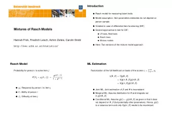
Mixtures of Rasch Models with R Package psychomix Hannah Frick, - - PowerPoint PPT Presentation

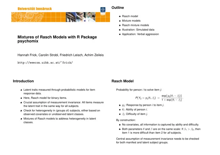
Mixtures of Rasch Models with R Package psychomix

Hannah Frick, Carolin Strobl, Friedrich Leisch, Achim Zeileis http://eeecon.uibk.ac.at/~frick/

Outline

Rasch model Mixture models Rasch mixture models Illustration: Simulated data Application: Verbal aggression

Introduction

Latent traits measured through probabilistic models for item response data. Here, Rasch model for binary items. Crucial assumption of measurement invariance: All items measure the latent trait in the same way for all subjects. Check for heterogeneity in (groups of) subjects, either based on

• bserved covariates or unobserved latent classes.

Mixtures of Rasch models to address heterogeneity in latent classes.

Rasch Model

Probability for person i to solve item j: P(Yij = yij|θi, βj) = exp{yij(θi − βj)} 1 + exp{θi − βj}. yij: Response by person i to item j.

θi: Ability of person i. βj: Difficulty of item j.

By construction: No covariates, all information is captured by ability and difficulty. Both parameters θ and β are on the same scale: If β1 > β2, then item 1 is more difficult than item 2 for all subjects. Central assumption of measurement invariance needs to be checked for both manifest and latent subject groups.

Rasch Model: Estimation

Joint estimation of θ and β is inconsistent. Conditional ML estimation: Use factorization of the full likelihood

• n basis of the scores ri = m

j=1 yij:

L(θ, β)

=

f(y|θ, β)

=

h(y|r, θ, β)g(r|θ, β)

=

h(y|r, β)g(r|θ, β). Estimate β from maximization of h(y|r, β). Also maximizes L(θ, β) if g(r|·) is assumed to be independent of θ and β; but potentially depending on auxiliary parameters δ: g(r|δ).

Mixture Models

Assumption: Data stems from different classes but class membership is unknown. Modeling tool: Mixture models. Mixture model = weight × component. Components represent the latent classes. They are densities or (regression) models. Weights are a priori probabilities for the components/classes, treated either as parameters or modeled through concomitant variables.

Rasch Mixture Models: Framework

Full mixture: Weights: Either (non-parametric) prior probabilities πk or weights π(k|x, α) based on concomitant variables x, e.g., a multinomial logit model. Components: Conditional likelihood for item parameters and specification of score probabilities f(y|π, α, β, δ) =

n

• i=1

K

• k=1

π(k|xi, α) h(yi|ri, βk) g(ri|δk).

Estimation of all parameters via ML through the EM algorithm.

Rasch Mixture Models: Score Probabilities

Original proposition by Rost (1990): Discrete distribution with parameters (probabilities) g(r) = Ψr. Number of parameters necessary is potentially very high: (number of items - 1) × (number of components). More parsimonious: Assume parametric model on score probabilities, e.g., using mean and variance parameters. General approach: Conditional logit model encompassing the

• riginal saturated parameterization and a mean/variance

parameterization (with only two parameters per component) as special cases g(r|δ) = exp{z⊤

r δ}

m−1

j=1 exp{z⊤ j δ}

.

Rasch Mixture Models: Score Probabilities

Motivation: When checking for measurement invariance, items are of interest, not the scores. Idea: Use g(r) = constant Equivalent to: Score distribution is the same over all components. Interpretation: Score distribution is irrelevant to the mixture. Consequently, the mixture is only influenced by latent classes regarding the item parameters. Differences in the score distribution (if any) do not influence the mixture, neither if coincident with differences in the item parameters nor if w.r.t. other classes.

Rasch Mixture Models: Score Models

Mean/variance: Parsimonious: 2 parameters per class. Mixture might catch on to latent score groups, even when no differential item functioning (DIF) is present. Saturated: Non-identified if no DIF present, as a mixture of multinomial models is itself a multinomial model. Possibly too many parameters to detect moderate DIF . Constant: Mixture only influenced by latent groups in items (i.e., DIF), yet parsimonious. Potentially less accurate if latent groups are present in both scores and items – and the groups coincide. Trade accuracy for robustness.

Software

Available in R in package psychomix at

http://CRAN.R-project.org/package=psychomix

Based on package flexmix (Grün and Leisch, 2008) for flexible estimation of mixture models. Based on package psychotools for estimation of Rasch models. Frick et al. (2011), provides implementation details and hands-on practical guidance. See also vignette("raschmix", package

= "psychomix").

Illustration: No DIF

Data generating process: m = 20 items, n = 100 subjects. No DIF: all item difficulties β = 0. Differences in scores through 2 different abilities: {−1.8, 1.8}.

scores Percent of Total

20 40 60 5 10 15 20

1

5 10 15 20

2

Illustration: No DIF

• meanvar score model

number of components

• AIC

BIC

• 1

2 2000 2040 2080

• constant score model

number of components

• AIC

BIC

• 1

2 2060 2100 2140

Figure: Mixture Rasch model with 1 to 2 classes and a meanvar (left) and a constant (right) specification of the score model.

Illustration: No DIF

Items Centered item difficulty parameters −2.0 −1.0 0.0 0.5

• ●
• ●
• ●
• ● ● ● ● ●
• 1

5 10 15 20

• Comp. 1
• Comp. 2

scores Density 5 10 15 20 0.00 0.10 0.20 0.30

Figure: Estimated item parameters (left) and score probabilities with empirical score distribution (right) of the 2-class Rasch mixture model with a meanvar score specification.

Illustration: Moderate DIF

Data generating process: m = 20 items, n = 1000 subjects. 2 items with DIF: β = (−1.2, 1.2) and β = (1.2, −1.2), all other items with β = 0. All abilities θ = 0.

Items Item difficulty −1.5 −0.5 0.5 1.5

• 1

5 10 15 20 Items Item difficulty −1.5 −0.5 0.5 1.5

• 1

5 10 15 20 Items Item difficulty −1.5 −0.5 0.5 1.5

• 1

5 10 15 20

Figure: Estimated item difficulties for whole sample and in both subsamples.

Illustration: Moderate DIF

• saturated score model

number of components

• AIC

BIC

• 1

2 27700 27850 28000

• constant score model

number of components

• AIC

BIC

• 1

2 29150 29250

Figure: Mixture Rasch model with 1 to 2 classes and a saturated (left) and a constant (right) specification of the score model.

Illustration: Moderate DIF

Items Item difficulty −1 1 2 3

• ● ●
• ● ● ● ●
• ●
• ●
• ● ● ● ● ● ● ● ● ● ● ●
• ● ●

1 5 10 15 20

• Comp. 1
• Comp. 2

Figure: Estimated item difficulties in a 2-class Rasch mixture model with a constant score model.

Application: Verbal Aggression Data

Behavioral study of psychology students: 243 women and 73 men. Description of frustrating situations:

S1: A bus fails to stop for me. S2: I miss a train because a clerk gave me faulty information.

Behavioral mode: Want or do. Verbally aggressive response: Curse, scold, or shout. 12 resulting items: S1WantCurse, S1DoCurse, S1WantScold, . . . , S2WantShout, S2DoShout Covariates: Gender and an anger score.

Verbal Aggression: Analysis

Fit model:

R> set.seed(1) R> mix <- raschmix(resp2 ~ 1, data = va12, k = 1:4, + scores = "constant", nrep = 5) R> mixC <- raschmix(resp2 ~ gender + anger, data = va12, + k = 2:4, scores = "constant", nrep = 5)

Select model:

R> rbind(mix = BIC(mix), mixC = c(NA, BIC(mixC))) 1 2 3 4 mix 3881.065 3854.193 3847.796 3865.268 mixC NA 3861.127 3850.129 3867.554 R> va12_mix <- getModel(mixC, which = "3")

Plot item profiles and effects of concomitant variables:

R> xyplot(va12_mix) R> effectsplot(va12_mix)

Verbal aggression: Item profiles

Item Centered item difficulty parameters

−2 2 4 1 2 3 4 5 6 7 8 9 10 11 12

• Comp. 1

1 2 3 4 5 6 7 8 9 10 11 12

• Comp. 2

1 2 3 4 5 6 7 8 9 10 11 12

• Comp. 3

Figure: Item difficulty profiles for the 3-component Rasch mixture model. Items 1–6: Situation S1 (bus). Items 7–12: Situation S2 (train). Order: want/do curse, want/do scold, want/do shout.

Verbal aggression: Effects displays

gender effect plot

gender Component (probability)

0.2 0.3 0.4 0.5 0.6 female male

• Component

1 2 3

• anger effect plot

anger Component (probability)

0.1 0.2 0.3 0.4 0.5 0.6 10 15 20 25 30 35

Component 1 2 3

Figure: Effect plots for the concomitant variables gender and age in a 3-component Rasch mixture model.

Verbal Aggression: Summary

Number of components: 3 different sets of item parameters necessary. Relationship between items differs between the latent classes. For shouting: Want is less extreme than do. For cursing and scolding, this depends on the latent class. One class does not differentiate much between the items, for the two other classes, cursing/scolding/shouting is increasingly extreme. Some dependence on covariates gender and anger score (albeit slightly poorer BIC).

Summary

Mixture Rasch models are a flexible means to check for measurement invariance. General framework incorporates concomitant variable models for mixture weights along with various score models. Newly introduced constant score model: robust and parsimonious. Implementation in R package psychomix.

References

Frick H, Strobl C, Leisch F , Zeileis A (2011). “Flexible Rasch Mixture Models with Package psychomix.” Working Paper 2011-21, Working Papers in Economics and Statistics, Research Platform Empirical and Experimental Economics, Universität Innsbruck.

http://EconPapers.RePEc.org/RePEc:inn:wpaper:2011-21

Fischer GH, Molenaar IW (eds.) (1995). Rasch Models: Foundations, Recent Developments, and Applications. Springer-Verlag, New York. Grün B, Leisch F (2008). "FlexMix Version 2: Finite Mixtures with Concomitant Variables and Varying and Constant Parameters." Journal of Statistical Software, 28(4), 1–35. http://www.jstatsoft.org/v28/i04/ Rost J (1990). “Rasch Models in Latent Classes: An Integration of Two Approaches to Item Analysis.” Applied Psychological Measurement, 14(3), 271–282.