Mixed Models II - Behind the Scenes Report Revised June 11, 2002 by - PDF document
Mixed Models II - Behind the Scenes Report Revised June 11, 2002 by G. Monette What is a mixed model "really" estimating? Paradox lost - paradox regained - paradox lost again. "Simple example": 4 patients each observed
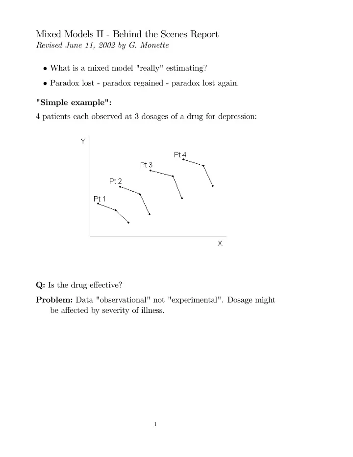
Mixed Models II - Behind the Scenes Report Revised June 11, 2002 by G. Monette • What is a mixed model "really" estimating? • Paradox lost - paradox regained - paradox lost again. "Simple example": 4 patients each observed at 3 dosages of a drug for depression: Q: Is the drug effective? Problem: Data "observational" not "experimental". Dosage might be affected by severity of illness. 1
OLS approaches : 1) Pooled (ignore subjects) ∴ Drug bad Model: Y ∼ X 2) Aggregate + regress Model ¯ Y ∼ ¯ X By Subject ∴ Drug even worse 2
3) Within Subject Y ∼ X + Sub ∴ Drug is good Note: • 2 ∼ ecological correlation • 2 vs 3: Robinson’s Paradox e.g. Life Expectancy vs. Smoking aggregated by country • 1 vs 3: Simpson’s Paradox Call � slope in 1. γ Pooled ˆ 2. γ Between ˆ 3. γ Within ˆ Let W B be weight (precision) of ˆ γ B W W be weight (precision) of ˆ γ W γ P = ( W B + W W ) − 1 ( W B ˆ Then ˆ γ B + W W ˆ γ W ) 3
So, ˆ γ P is an optimal combination of ˆ γ B and ˆ γ W Note: "optimal" in common model is connect. In our example ˆ γ W is probably a "good" estimator, ˆ γ B is NOT. So, ˆ γ P mixes the good and the bad. What does a Mixed Model do? Does it give us ˆ γ W ? Or ˆ γ P ? Answer: Something in between. With a random intercept model: Y ∼ X / ∼ 1 | Sub γ MM is also an "optimal" combination of ˆ ˆ γ W and ˆ γ B If Y i j = γ 00 + γ 10 X i j + u 0 j + ε i j ↓ ↓ σ 2 V ar : τ 00 then, σ 2 /n Weight on ˆ γ B = × OLS weight σ 2 /n + τ 00 Weight on ˆ γ W = OLS weight I.E. � � σ 2 /n γ MM = ( · · · ) − 1 × ˆ W B ˆ γ B + W W ˆ γ W σ 2 /n + τ 00 Note: Here n is # of obs/subject. So, � � σ 2 /n γ MM = ( · · · ) − 1 × ˆ W B ˆ γ B + W W ˆ γ W σ 2 /n + τ 00 If σ 2 /n very small / τ 00 ( ∼ 0) ” ” ” ” = ∼ ˆ γ W 4
If σ 2 /n big / τ 00 ( ∼ 1) ” ” ” ” = ∼ ˆ γ P γ MM is between ˆ γ W depending on σ 2 / ( nτ 00 ) So ˆ γ P and ˆ If the between subject effect is not the same as the within subject effect (often the case with observational data) then Mixed Model can give biased results. In our example: 5
To the Rescue: Contextual variable and within subject effects. Idea: decompose X i j : X i j = ¯ X · j + ( X i j − ¯ X · j ) � �� � ↑ ↑ mean within S deviation from within subject mean Use ¯ X · j as a level-2 variable and X i j − ¯ X · j as a level-1 variable Consider OLS: E ( Y ) = γ 0 + γ 1 ¯ X · j + γ 2 ( ¯ X i j − ¯ X · j ) What is γ 1 ? △ E ( Y ) / △ ¯ X · j when X i j − ¯ X · j = 0 i.e. between S effect when X i j = ¯ X · j What is γ 2 ? Answer: ˆ γ 2 = ˆ γ W ! 6
So a possible approach for Mixed Models: 1. Transform inner variables into outer means and inner deviations. Handy trick for small datasets: PROC GLM; CLASS SUB; OUTPUT OUT = dsname P = X_B R = X_W; 2. Model with both 3. Test equality of parameters. If equal can revert to raw inner variable. 4. If not equal, rich possibilities for interpretation. Note: Much discussion on "centering" • Should we use X i j − ¯ X · j or X i j − ¯ X • Often seems inconclusive. [See centering on � X min in next section] Problem: • Centering X i j defines γ for ¯ X · j • has little effect on γ for X i j - "center" !! Essentially 1. Controlling for ¯ X · j defines γ for X i j − whatever 2. Controlling for X i j − whatever defines γ for ¯ X · j Compositional vs contextual effects We have three variable to consider (note that we can start with GMC (grand mean centering) of X ij . This only affect the meaning of the intercept (and effects of other interacting variables) but does affect the effects below. 3 variables: 7
1. X ij (raw variables) 2. X ij − X · j (CWC: centered within contexts) 3. X · j (contextual mean) Note that we can’t use all 3 variables (why not?) 3 effects: 1. γ W within context 2. γ B between contexts = compositional effect 3. γ C contextual effect Diagram: (R&B p. 140) γ B = γ W + γ C How to get what: Raw CWC Mean Variables: X ij X ij − X · j X · j Contextual model: γ W — γ C Compositional model: — γ W γ B 8
Hausman specification test: (S&B p. 87) • Random vs Fixed: Is � γ X in random intercept model an unbiased estimator of γ W ? • Idea: equivalent to testing γ C = 0 . — If so, then γ B = γ W and random intercept model is ok. — If not, then use ’fixed effects’ model. — Third choice: use contextual or compositional model. Contextual or compositional? • Fixed part is equivalent (same except for labelling of effects) since X C = X B A for some non-singular matrix A . Equivalently we note that span ( X C ) = span ( X B ) • But the random part is different. Two random models are equiv- alent if there is a single A such Z Cj = Z Bj A Consider using X ij − X · j and 1 in the random model instead of X ij and 1 : Two solutions: 9
1. Choose according to desired random model. (S&B prefer contex- tual, p. 80ff.) Then estimate desired parameters with ESTIMATE statements. 2. Choose variables for fixed part to get estimates you want. Choose variables for random part according to desired pattern of vari- ance. Variables don’t have to be the same! As long as the fixed model is equivalent to a model with the random effects, then the models are equivalent. 10
Multivariate EBLUPs eg. β 0 j = γ 00 − u 0 j β 1 j = γ 10 − u 1 j with: Let be OLS estimation of 11
Combine OLS with Empirical Prior Amount and direction of shrinkage depends on shape of T. Note what happens if we drop a random effect: Note: Shrinkage of works the same way. Just centre picture at Note: If T is "small" in some direciton, collapse into T . 12
’Appendix’: Creating contextual variables in large data sets: Suppose we want to create a contextual variable and a within-cluster deviation for a variable X DATA MYDATA; INPUT GROUP X; CARDS; 1 10 1 20 1 30 2 0 2 10 2 20 3 40 3 50 ;; PROC MEANS; BY GROUP; VAR X; OUPUT OUT=NEW MEAN = M; RUN; DATA NEW; SET NEW; KEEP M GROUP; DATA TOGETHER; MERGE MYDATA NEW; BY GROUP; RUN; PROC PRINT DATA TOGETHER; RUN; 13
Recommend
More recommend
Explore More Topics
Stay informed with curated content and fresh updates.
