MITOCW | watch?v=Q2qjnLO3I_M The following content is provided under - PDF document
MITOCW | watch?v=Q2qjnLO3I_M The following content is provided under a Creative Commons license. Your support will help MIT OpenCourseWare continue to offer high-quality educational resources for free. To make a donation, or to view additional
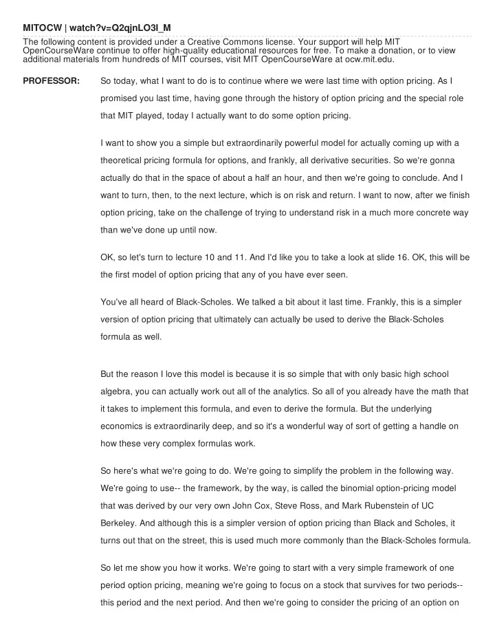
MITOCW | watch?v=Q2qjnLO3I_M The following content is provided under a Creative Commons license. Your support will help MIT OpenCourseWare continue to offer high-quality educational resources for free. To make a donation, or to view additional materials from hundreds of MIT courses, visit MIT OpenCourseWare at ocw.mit.edu. PROFESSOR: So today, what I want to do is to continue where we were last time with option pricing. As I promised you last time, having gone through the history of option pricing and the special role that MIT played, today I actually want to do some option pricing. I want to show you a simple but extraordinarily powerful model for actually coming up with a theoretical pricing formula for options, and frankly, all derivative securities. So we're gonna actually do that in the space of about a half an hour, and then we're going to conclude. And I want to turn, then, to the next lecture, which is on risk and return. I want to now, after we finish option pricing, take on the challenge of trying to understand risk in a much more concrete way than we've done up until now. OK, so let's turn to lecture 10 and 11. And I'd like you to take a look at slide 16. OK, this will be the first model of option pricing that any of you have ever seen. You've all heard of Black-Scholes. We talked a bit about it last time. Frankly, this is a simpler version of option pricing that ultimately can actually be used to derive the Black-Scholes formula as well. But the reason I love this model is because it is so simple that with only basic high school algebra, you can actually work out all of the analytics. So all of you already have the math that it takes to implement this formula, and even to derive the formula. But the underlying economics is extraordinarily deep, and so it's a wonderful way of sort of getting a handle on how these very complex formulas work. So here's what we're going to do. We're going to simplify the problem in the following way. We're going to use-- the framework, by the way, is called the binomial option-pricing model that was derived by our very own John Cox, Steve Ross, and Mark Rubenstein of UC Berkeley. And although this is a simpler version of option pricing than Black and Scholes, it turns out that on the street, this is used much more commonly than the Black-Scholes formula. So let me show you how it works. We're going to start with a very simple framework of one period option pricing, meaning we're going to focus on a stock that survives for two periods-- this period and the next period. And then we're going to consider the pricing of an option on
that stock that expires next period. We're going to figure out what the price is this period. So we've got a stock XYZ, and let's suppose the current stock price is S0. And let's suppose that we have a call option on this stock with a strike price of K, and where the option expires tomorrow. And so tomorrow's value of the option is simply equal to C1, which is the maximum of tomorrow's stock price minus the strike, or 0, the bigger of those two. That's the payoff for the call option. And the question that we want to attack is, what is the option's price today? In other words, what is C0? So we draw a timeline, as I've told you, for every one of these problems. Draw a timeline just so that there's no confusion. So tomorrow, the stock price is going to be worth S1, and the option price is just equal to C1, which is the payoff, since it expires tomorrow. And the payoff is just the maximum of S1 minus K and 0. And the object of our focus is to try to figure out what the value of the option is today. And so I'm going to argue that if we can figure out what it is today, based upon this, then we can actually generalize it in a very natural way to figure out what the price is for any number of periods in the future. So how do we do that? Well, we first have to make an assumption about how the stock price behaves. As I mentioned last time, we need to say something about the dynamics of stock prices, and remember that Bachelier, that French mathematician that came up with a rudimentary version of an option pricing formula in 1900, he developed the mathematics for Brownian motion, or a random walk, for the particular stock price. So you have to assume something about how the stock price moves. So what we're going to do in a simplified version is to assume that the stock price tomorrow is a coin flip. It's a Bernoulli trial. That's the technical term. So it either goes up or down. And if it goes up, it goes up by a gross amount u. So the value of the stock tomorrow, S1, is going to be equal to u multiplied by S0. So if it goes up by 10% tomorrow, then u is equal to 1.1. Or it can go down by a factor of d tomorrow, and so if it goes down by 10%, then d is 0.9. So we're going to simply assert that this is the statistical behavior of stock prices. Now, granted, this is a very, very strong simplification, but bear with me. After I derive the simple version of the pricing formula, I'm going to show you how to make it much, much more
complex. And the additional complexity will be really simple to achieve once we understand this very basic version. Now, the probability of going up or down is not 50/50-- doesn't have to be 50/50. So I'm going to assert that it's equal to some probability of p and 1 minus p. So it either goes up by p or goes down with probability 1 minus p, and the amount that it goes up or down is given by u and d. And I'm going to assert that u is greater than d. Question? AUDIENCE: So u and d are not the changes, but you're just assuming that, in your case, [INAUDIBLE]. PROFESSOR: Sorry, that they're-- AUDIENCE: It's not necessary to always use [INAUDIBLE] d, or can you assume-- PROFESSOR: Yeah, I'm assuming as a matter of normalization that u is greater than d. It doesn't matter. I mean, one thing has to be bigger than the other, so I just may as well assume that u is greater than d. Yeah, question? AUDIENCE: Is it necessary to add up to 1 [INAUDIBLE]? PROFESSOR: u and do don't have to add up to anything. That's right. p and 1 minus p always add up to 1, right. So for example, if this is a growth stock that's really doing well, then u may be 1.1, 10%, and d may be 0.99. So in other words, when it goes down, it goes down by 1%. When it goes up, it goes up by 10%. So on average, when you multiply by p, 1 minus p, depending on what they are, you can get a stock that's got a positive drift. If, on the other hand, you've got a stock that's declining in value, then it may end up that d much smaller than u, and 1 minus p is bigger than p, which means that you're more likely to be going down than you are going up. So it's pretty general. Yeah? AUDIENCE: u is bigger than 1 and d is lower than 1, or you could [INAUDIBLE]? PROFESSOR: It doesn't have to be. But typically you would think that in the up state, it's going to be bigger than 1, and the down state, it will be less than 1. But it doesn't have to be. What I'm going to normalize it to be is u is greater than d. And later on, we may make some other economic assumptions that I'll come to that will tell you a little bit more about what u and d are. Now, if it's true that the stock price can only take on two values tomorrow, then it stands to reason that the option can only take on two values tomorrow. And those are the two values.
reason that the option can only take on two values tomorrow. And those are the two values. It's going to be Cu and Cd. Cu is where the stock price goes up to u times S0. Therefore, the option's going to be worth u S0 minus K, 0, maximum of those two. And similarly, if it turns out that the stock price goes down tomorrow, then the option is worth this tomorrow. Two values for the stock tomorrow implies two values for the option tomorrow. Any questions about that? OK, so having said that, we can now proceed to ask the question, given this simple framework, what should the option price today depend on? It's going to be a function of a bunch of parameters. So what should it depend upon? Well, the parameters that are given are these-- the stock price today, the strike price, u and d, p, and the interest rate between today and tomorrow. Those are the only parameters that we have. These are it. This is everything. It's going to turn out that with the simple framework that I've put down, we will be able to derive a closed-form analytical expression for what the option price has to be today-- C0. I'm going to do that for you in just a minute. But it's going to turn out that that option pricing formula, that f of stuff, is going to depend on all of these parameters except for one. One of these parameters is going to drop out. In other words, one of these parameters is redundant. And anybody want to take a guess as to what that parameter might be? What parameter do you think might not matter for pricing an option? Yeah, Terry. AUDIENCE: The interest rate, the r? PROFESSOR: The interest rate. Well, that's a good guess, but that's not the case. That's what I would have guessed, because that seems to be the thing that should matter the least, given how important all of these other parameters are. Anybody want to take another guess? Yeah, Ken. AUDIENCE: Today's stock price. PROFESSOR: Today's stock price. That's another good guess. [LAUGHTER]
Recommend
More recommend
Explore More Topics
Stay informed with curated content and fresh updates.


