
Mining Distance-Based Outliers in Near Linear Time with - PowerPoint PPT Presentation
Mining Distance-Based Outliers in Near Linear Time with Randomization and a Simple Pruning Rule Stephen D. Bay 1 and Mark Schwabacher 2 1 Institute for the Study of Learning and Expertise sbay@apres.stanford.edu 2 NASA Ames Research Center
Mining Distance-Based Outliers in Near Linear Time with Randomization and a Simple Pruning Rule Stephen D. Bay 1 and Mark Schwabacher 2 1 Institute for the Study of Learning and Expertise sbay@apres.stanford.edu 2 NASA Ames Research Center Mark.A.Schwabacher@nasa.gov
Motivation Detecting outliers or anomalies is an important KDD task with many practical applications and fast algorithms are needed for large databases. In this talk, I will – Show that very simple modifications of a basic algorithm lead to extremely good performance – Explain why this approach works well – Discuss limitations of this approach
Distance-Based Outliers • The main idea is to find points in low density regions of the feature space k ≅ P x ( ) NV • V is the total volume within radius d • N is the total number of x d examples • k is the number of examples in sphere Distance measure determines proximity and scaling.
Outlier Definitions • Outliers are the examples for which there are fewer than p other examples within distance d – Knorr & Ng • Outliers are the top n examples whose distance to the kth nearest neighbor is greatest – Ramaswamy, Rastogi, & Shim • Outliers are the top n examples whose average distance to the k nearest neighbors is greatest – Angiulli & Pizzuti, Eskin et al. k ≅ ( ) P x These definitions all relate to NV
Existing Methods • Nested Loops – For each example, find it’s nearest neighbors with a sequential scan • O(N 2 ) • Index Trees – For each example, find it’s nearest neighbors with an index tree • Potentially N log N, in practice can be worse than NL • Partitioning Methods – For each example, find it’s nearest neighbors given that the examples are stored in bins (e.g., cells, clusters) • Cell-based methods potentially N, in practice worse than NL for more than 5 dimensions (Knorr & Ng) • Cluster based methods appear sub-quadratic
Our Algorithm • Based on Nested loops – For each example, find it’s nearest neighbors with a sequential scan • Two modifications – Randomize order of examples • Can be done with a disk-based algorithm in linear time – While performing the sequential scan, • Keep track of closest neighbors found so far • prune examples once the neighbors found so far indicate that the example cannot be a top outlier • Process examples in blocks • Worst case O(N 2 ) distance computations, O(N 2 /B) disk accesses
Pruning • Outliers based on distance to the 3rd nearest neighbor (k=3) d is distance to 3 rd nearest sequential 39 State-gov 77516 Bachelors 13 50 Self-emp-not-inc 83311 Bachelors 13 38 Private 215646 HS-grad 9 scan neighbor for the weakest top 53 Private 234721 11th 7 28 Private 338409 Bachelors 13 outlier 37 Private 284582 Masters 14 49 Private 160187 9th 5 52 Self-emp-not-inc 209642 HS-grad 9 31 Private 45781 Masters 14 42 Private 159449 Bachelors 13 37 Private 280464 Some-college 10 30 State-gov 141297 Bachelors 13 23 Private 122272 Bachelors 13 32 Private 205019 Assoc-acdm 12 40 Private 121772 Assoc-voc 11 34 Private 245487 7th-8th 4 x 25 Self-emp-not-inc 176756 HS-grad 9 d 32 Private 186824 HS-grad 9 38 Private 28887 11th 7 43 Self-emp-not-inc 292175 Masters 14 40 Private 193524 Doctorate 16 54 Private 302146 HS-grad 9 35 Federal-gov 76845 9th 5 43 Private 117037 11th 7 59 Private 109015 HS-grad 9 56 Local-gov 216851 Bachelors 13 19 Private 168294 HS-grad 9 54 ? 180211 Some-college 10 39 Private 367260 HS-grad 9
Experimental Setup • 6 data sets varying from 68K to 5M examples • Mixture of discrete and continuous features (23- 55) • Wall time reported (CPU + IO) – Time does not include randomization • No special caching of records • Pentium 4, 1.5 Ghz, 1GB Ram • Memory footprint ~3MB • Mined top 30 outliers, k=5, block size = 1000, average distance
Scaling with N C o re l H is to g ra m C o re l H is to g ra m K D D C u p 1 9 9 9 K D D C u p 1 9 9 9 4 8 1 0 1 0 3 6 1 0 1 0 2 4 1 0 1 0 Total Time Total Time 1 2 1 0 1 0 0 0 1 0 1 0 -1 -2 1 0 1 0 3 4 5 3 4 5 6 7 1 0 1 0 1 0 1 0 1 0 1 0 1 0 1 0 S iz e S iz e P e rs o n P e rs o n N o rm a l 3 0 D N o rm a l 3 0 D 8 6 1 0 1 0 6 4 1 0 1 0 Total Time Total Time 4 2 1 0 1 0 0 2 1 0 1 0 0 -2 1 0 1 0 3 4 5 6 7 3 4 5 6 1 0 1 0 1 0 1 0 1 0 1 0 1 0 1 0 1 0 S iz e S iz e
Scaling Summary Data Set Slope Corel Histogram 1.13 Covertype 1.25 KDDCup 1999 1.13 Household 1990 1.32 Person 1990 1.16 Normal 30D 1.15 Slope of regression fit relating log time to log N = + = b log log log or t a b N t aN
Scaling with k P e rs o n P e rs o n N o rm a l 3 0 D N o rm a l 3 0 D 4 5 0 0 4 5 0 0 4 0 0 0 4 0 0 0 3 5 0 0 3 5 0 0 Total Time Total Time 3 0 0 0 3 0 0 0 2 5 0 0 2 5 0 0 2 0 0 0 2 0 0 0 0 2 0 4 0 6 0 8 0 1 0 0 0 2 0 4 0 6 0 8 0 1 0 0 K K 1 million records used for both Person and Normal 30D
Average Case Analysis Consider operation of the algorithm at moment in time – Outliers defined by distance to kth neighbor – Current cutoff distance is d – Randomization + sequential scan = I.I.D. sampling of pdf Let p(x) = prob. randomly drawn example lies within distance d ( ) ∫ = p x pdf ( x ) dV x d How many examples do we need to look at?
For non-outliers, number of samples follows a negative binomial distribution. Let P(Y=y) be probability of obtaining kth success on step y − y 1 = = − − k y k P ( Y y ) p ( x ) ( 1 p ( x )) − k 1 Expectation of number of samples with infinite data is ∞ [ ] = ∑ = ⋅ E Y P ( Y y ) y = y k [ ] k = E Y p ( x )
How does the cutoff change during program execution? Person 7 6 5 4 Cutoff 3 2 50K 100K 1 1M 5M 0 0 20 40 60 80 100 Percent of Data Set Processed
Scaling Rate b Versus Cutoff Ratio 1.8 Uniform 3D 1.6 Polynomial scaling b 1.4 Household Covertype Person 1.2 KDDCup Corel Histogram Mixed 3D Normal 30D 1 0.2 0.4 0.6 0.8 1 1.2 Relative change in cutoff (50K/5K) as N increases
Limitations • Failure modes – examples not in random order – examples not independent – no outliers in data
Method fails when there are no outliers Unifo rm 3 D Unifo rm 3 D 6 1 0 b=1.76 4 1 0 P ( x ) Total Time i 2 1 0 0 1 0 -2 1 0 3 4 5 6 1 0 1 0 1 0 1 0 S iz e Examples drawn from a uniform distribution in 3 dimensions
However, the method is efficient if there are at least a few outliers M ixe d 3 D M ixe d 3 D 6 1 0 b=1.11 4 1 0 P ( x ) Total Time i 2 1 0 0 1 0 -2 1 0 3 4 5 6 1 0 1 0 1 0 1 0 S iz e Examples drawn from 99% uniform, 1% Gaussian distribution
Future Work • Pruning eliminates examples when they cannot be a top outlier. Can we prune examples when they are almost certain to be an outlier? • How many examples is enough? Do we need to do the full N 2 comparisons? • How do algorithm settings affect performance and do they interact with data set characteristics? • How do we deal with dependent data points?
Summary & Conclusions • Presented a nested loop approach to finding distance-based outliers • Efficient and allows scaling to larger data sets with millions of examples and many features • Easy to implement and should be the new strawman for research in speeding up distance-based outliers
Resources • Executables available from http://www.isle.org/~sbay • Comparison with GritBot on Census data http://www.isle.org/~sbay/papers/kdd03/ • Datasets are public and are available by request
Scaling Summary N b=1.13 b=1.32 NlogN 100 1.8 4.4 2 1000 2.5 9.1 3 10000 3.3 19.1 4 100000 4.5 39.8 5 1000000 6.0 83.2 6 10000000 8.1 173.8 7
How big a sample do we need? It depends… N o rm a l3 0 d - k1 0 0 a 5 0 0 N o rm a l3 0 d - k1 0 0 a 5 0 0 P e rs o n - k30 a 3 0 P e rs o n - k30 a 3 0 1 1 0.8 0.8 Correspondence Correspondence 0.6 0.6 0.4 0.4 0.2 0.2 0 0 3 4 5 6 3 4 5 6 7 1 0 1 0 1 0 1 0 1 0 1 0 1 0 1 0 1 0 S iz e o f re fe re n c e s e t S iz e o f re fe re n c e s e t
Recommend


More recommend
Explore More Topics
Stay informed with curated content and fresh updates.