Detecting Outliers in HMM modeling through Relative Entropy with - PowerPoint PPT Presentation
Detecting Outliers in HMM modeling through Relative Entropy with Applications to Change-Point Detection V. Perduca, G. Nuel JOBIM 2012 V. Perduca (MAP 5 - Paris Descartes) Detecting Outliers in HMM modeling JOBIM 2012 1 / 17 Change-point
Detecting Outliers in HMM modeling through Relative Entropy with Applications to Change-Point Detection V. Perduca, G. Nuel JOBIM 2012 V. Perduca (MAP 5 - Paris Descartes) Detecting Outliers in HMM modeling JOBIM 2012 1 / 17
Change-point detection, HMMs and outliers ◮ Given an heterogeneous sequence: find the segments in which the signal is homogeneous ◮ Here: Hidden Markov modeling ◮ Segmentation models are sensitive to the presence of outliers No outliers With outliers ● 100 100 ● ● ● ● ● 50 50 ● ● ● ● ● ● ● ● ● ● ● ● X X ● ● ● ● ● ● ● ● 0 0 ● ● ● ● ● ●● ● −50 −50 ● 0 200 400 600 800 1000 0 200 400 600 800 1000 Index Index V. Perduca (MAP 5 - Paris Descartes) Detecting Outliers in HMM modeling JOBIM 2012 2 / 17
Hidden Markov Models ◮ X i observed variable ◮ S i hidden variable, for i = 1 . . . , n S 1 S 2 S 3 S 4 S 5 X 1 X 2 X 3 X 4 X 5 Factorization of the joint probability distribution n � P ( S i = s i | S i − 1 = s i − 1 ) P ( S 1: n = s 1: n , X 1: n = x 1: n ) = P ( S 1 = s 1 ) i =2 n � P ( X i = x i | S i = s i ) i =1 V. Perduca (MAP 5 - Paris Descartes) Detecting Outliers in HMM modeling JOBIM 2012 3 / 17
Hidden Markov Models ◮ X i observed variable ◮ S i hidden variable, for i = 1 . . . , n S 1 S 2 S 3 S 4 S 5 X 1 X 2 X 3 X 4 X 5 Factorization of the joint probability distribution n n � � P ( S 1: n , X 1: n ) = P ( S 1 ) P ( S i | S i − 1 ) P ( X i | S i ) i =2 i =1 V. Perduca (MAP 5 - Paris Descartes) Detecting Outliers in HMM modeling JOBIM 2012 3 / 17
Hidden Markov Models ◮ X i observed variable ◮ S i hidden variable, for i = 1 . . . , n S 1 S 2 S 3 S 4 S 5 X 1 X 2 X 3 X 4 X 5 Factorization of the joint probability distribution n n � � P ( S 1: n , X 1: n ) = P ( S 1 ) P ( S i | S i − 1 ) P ( X i | S i ) i =2 i =1 Example (Application to change point detection) ◮ Level-based: S i = underlying level of observation X i ◮ Segment-based: S i = segment of X i with S 1 = 1 and S n = # segments V. Perduca (MAP 5 - Paris Descartes) Detecting Outliers in HMM modeling JOBIM 2012 3 / 17
Inference in HMMs If E = { X 1: n = x 1: n } observed, compute P ( E ) , P ( S i |E ) , P ( S i | S i − 1 , E ) ... Backward and Forward recursions (Baum-Welch algorithm) Standard inference problems solved by combining the Forward and Backward quantities ◮ F i ( S i ) := P ( S i , X 1: i = x 1: i ) ◮ B i ( S i ) := P ( X i +1: n = x i +1: n | S i ), which are computed recursively: ◮ F i ( S i ) = � S i − 1 F i − 1 ( S i − 1 ) P ( S i | S i − 1 ) P ( X i | S i ) ◮ B i − 1 ( S i − 1 ) = � S i P ( S i | S i − 1 ) P ( X i | S i ) B i ( S i ). E.g. P ( S i , E ) = F i ( S i ) B i ( S i ) Parameter estimation EM algorithm: Backward/Forward quantities provide explicit update formulas V. Perduca (MAP 5 - Paris Descartes) Detecting Outliers in HMM modeling JOBIM 2012 4 / 17
Ad hoc model for outlier detection in HMMs ◮ X i is an outlier if it is not generated by the underlying HMM ◮ ⇒ extend the HMM with variables for the outliers status [Shah 2006] Topology and conditional dependencies (homoscedastic Gaussian case) S 1 S 2 S 3 S 4 S 5 X 1 X 2 X 3 X 4 X 5 O 1 O 2 O 3 O 4 O 5 ◮ O i = 1 iff X i is outlier; P ( O i = 1) = ρ ◮ P ( S 1 ); P ( S i | S i − 1 ): same as for underlying HMM ◮ P ( X i | S i , O i = 0) = N ( µ S i , σ 2 ): same as for underlying HMM ◮ P ( X i | S i , O i = 1) = N ( µ S i , σ 2 ) + N (0 , δ 2 ) V. Perduca (MAP 5 - Paris Descartes) Detecting Outliers in HMM modeling JOBIM 2012 5 / 17
Inference in the ad hoc model Inferring outlier posterior probabilities � � ρ P ( X i = x i | S i , O i =1) P ( O i = 1 |E ) = � ρ P ( X i = x i | S i , O i =1)+(1 − ρ ) P ( X i = x i | S i , O i =0) · P ( S i |E ) S i where F i ( S i ) B i ( S i ) P ( S i |E ) = � S i F i ( S i ) B i ( S i ) � F i ( S i ) = F i − 1 ( S i ) P ( S i | S i − 1 ) P ( X i | S i ) S i − 1 V. Perduca (MAP 5 - Paris Descartes) Detecting Outliers in HMM modeling JOBIM 2012 6 / 17
Inference in the ad hoc model Inferring outlier posterior probabilities � � ρ P ( X i = x i | S i , O i =1) P ( O i = 1 |E ) = � ρ P ( X i = x i | S i , O i =1)+(1 − ρ ) P ( X i = x i | S i , O i =0) · P ( S i |E ) S i where F i ( S i ) B i ( S i ) P ( S i |E ) = � S i F i ( S i ) B i ( S i ) � � F i ( S i ) = F i − 1 ( S i ) P ( S i | S i − 1 ) P ( X i = x i | S i , O i = o ) P ( O i = o ) o =0 , 1 S i − 1 V. Perduca (MAP 5 - Paris Descartes) Detecting Outliers in HMM modeling JOBIM 2012 6 / 17
Inference in the ad hoc model Inferring outlier posterior probabilities � � ρ P ( X i = x i | S i , O i =1) P ( O i = 1 |E ) = � ρ P ( X i = x i | S i , O i =1)+(1 − ρ ) P ( X i = x i | S i , O i =0) · P ( S i |E ) S i where F i ( S i ) B i ( S i ) P ( S i |E ) = � S i F i ( S i ) B i ( S i ) � � F i ( S i ) = F i − 1 ( S i ) P ( S i | S i − 1 ) P ( X i = x i | S i , O i = o ) P ( O i = o ) o =0 , 1 S i − 1 � � P ( S i | S i − 1 ) P ( X i = x i | S i , O i = o ) P ( O i = o ) B i ( S i ) B i − 1 ( S i − 1 ) = o =0 , 1 S i V. Perduca (MAP 5 - Paris Descartes) Detecting Outliers in HMM modeling JOBIM 2012 6 / 17
EM algorithm for the ad hoc model Parameter updates: 2 new parameters ( ρ, δ 2 ) ◮ Transition parameters have same update formulas as in plain HMM � n i =1 P ( O i =1 |E ) ◮ ρ = n ◮ µ s , σ 2 , δ 2 found as fixed points: i x i [ P ( S i = s , O i =1 |E ) σ 2 + P ( S i = s , O i =0 |E )( σ 2 + δ 2 )] � µ s = i [ P ( S i = s , O i =1 |E ) σ 2 + P ( S i = s , O i =0 |E )( σ 2 + δ 2 )] � s ( x i − µ s ) 2 P ( S i = s , O i =0 |E ) � � σ 2 = i � � s P ( S i = s , O i =0 |E ) i s ( x i − µ s ) 2 P ( S i = s , O i =1 |E )) σ 2 + δ 2 � � = i � � s P ( S i = s , O i =1 |E ) i ρ P ( X i = x i | S i , O i =1) where P ( S i , O i |E ) = ρ P ( X i = x i | S i , O i =1)+(1 − ρ ) P ( X i = x i | S i , O i =0) · P ( S i |E ) Initialization k -means algorithm and z-score V. Perduca (MAP 5 - Paris Descartes) Detecting Outliers in HMM modeling JOBIM 2012 7 / 17
Validation of the ad hoc model on a toy example ◮ Simulations done with the homoscedastic Gaussian ad hoc model: ◮ H0: no outlier ( δ = 0) ◮ H1: presence of outliers ( δ � = 0) ◮ Global statistics: T = max i =1 ,..., n P ( O i = 1 |E ) ◮ P ( O i |E ) computed using the true parameters δ AUC ( T ) 0.00 0.52 [0.48,0.55] 0.50 0.49 [0.46,0.53] 1.00 0.56 [0.52,0.59] 1.50 0.74 [0.71,0.78] 2.00 0.87 [0.85,0.89] 2.50 0.93 [0.91,0.95] 3.00 0.97 [0.95,0.98] 3.50 0.99 [0.98,0.99] 4.00 0.99 [0.99,1.00] 4.50 0.99 [0.99,1.00] V. Perduca (MAP 5 - Paris Descartes) Detecting Outliers in HMM modeling JOBIM 2012 8 / 17
Application of the ad hoc model to real data ◮ CNV dataset from breast cancer cell line BT474 [Snijders 2001] ◮ Level-based model: S i = level of observation X i ◮ Parameters in the ad hoc model estimated with the EM algorithm Original data Original data 1.0 ● ● ● ● ● ● 0.5 30 ● ● ● ● ● ● ● ●● ● ● ● ● ●●● ● ● ● ●● ● ● ● ● ● ● ● ● ● ●●● ●●●● ● ● ●●● ● ●● ● ● ● ● ● ●●● ● ●●● ● ● ● ● ● ● ● ●● ● ● ●● ● ● ● ● ● ● 0.0 ● ● ● ●● ● −log(1 − post_out) ● ● ● ● ● ● ● ● ● 20 −0.5 X ● ● ● ●● ● ● ● ● ● ●● ● ●● ● ● ● ● −1.0 ● ● ● 10 −1.5 ● −2.0 0 0 20 40 60 80 100 120 0 20 40 60 80 100 120 Index Index V. Perduca (MAP 5 - Paris Descartes) Detecting Outliers in HMM modeling JOBIM 2012 9 / 17
Application of the ad hoc model to real data ◮ CNV dataset from breast cancer cell line BT474 [Snijders 2001] ◮ Level-based model: S i = level of observation X i ◮ Parameters in the ad hoc model estimated with the EM algorithm Original data with outliers Original data 1.0 ● ● ● ● ● ● 0.5 30 ● ● ● ● ● ● ● ●● ● ● ● ● ●●● ● ● ● ●● ● ● ● ● ● ● ● ● ● ●●● ●●●● ● ●●● ●● ● ● ● ● ● ●●● ● ●●● ● ● ● ● ● ● ● ●● ● ● ●● ● ● ● ● ● ● 0.0 ● ● ● ●● ● −log(1 − post_out) ● ● ● ● ● ● ● ● ● 20 −0.5 X ● ● ● ● ●● ● ● ● ● ●● ●● ● ● ● ● −1.0 ● ● ● 10 −1.5 ● −2.0 0 0 20 40 60 80 100 120 0 20 40 60 80 100 120 Index Index V. Perduca (MAP 5 - Paris Descartes) Detecting Outliers in HMM modeling JOBIM 2012 9 / 17
Recommend
More recommend
Explore More Topics
Stay informed with curated content and fresh updates.










![A Talk on Protein Homology Detection by HMM-HMM comparisons[1] Sding, J Qing Ye Department of](https://c.sambuz.com/139484/a-talk-on-protein-homology-detection-by-hmm-hmm-s.webp)
