min { a i , a j } max { a i , a j } P j P j P i P i P i P j Step 1 - PDF document
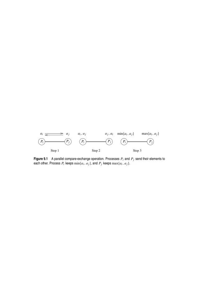
a i a j a i , a j a j , a i min { a i , a j } max { a i , a j } P j P j P i P i P i P j Step 1 Step 2 Step 3 Figure 9.1 A parallel compare-exchange operation. Processes P i and P j send their elements to each other. Process P i keeps min { a i ,
a i a j a i , a j a j , a i min { a i , a j } max { a i , a j } P j P j P i P i P i P j Step 1 Step 2 Step 3 Figure 9.1 A parallel compare-exchange operation. Processes P i and P j send their elements to each other. Process P i keeps min { a i , a j } , and P j keeps max { a i , a j } .
1 6 8 11 13 2 7 9 10 12 2 7 9 10 12 1 6 8 11 13 2 7 9 10 12 1 6 8 11 13 P j P j P i P i Step 1 Step 2 1 2 6 7 8 9 10 11 12 13 1 2 6 7 8 9 10 11 12 13 1 2 6 7 8 9 10 11 12 13 P j P j P i P i Step 3 Step 4 Figure 9.2 A compare-split operation. Each process sends its block of size n / p to the other process. Each process merges the received block with its own block and retains only the appropriate half of the merged block. In this example, process P i retains the smaller elements and process P j retains the larger elements.
x ′ = min { x , y } x ′ = min { x , y } x x y y y ′ = max { x , y } y ′ = max { x , y } (a) x ′ = max { x , y } x ′ = max { x , y } x x y y y ′ = min { x , y } y ′ = min { x , y } (b) Figure 9.3 A schematic representation of comparators: (a) an increasing comparator, and (b) a decreasing comparator.
Columns of comparators Interconnection network Input wires Output wires Figure 9.4 A typical sorting network. Every sorting network is made up of a series of columns, and each column contains a number of comparators connected in parallel.
Original sequence 3 5 8 9 10 12 14 20 95 90 60 40 35 23 18 0 1st Split 3 5 8 9 10 12 14 0 95 90 60 40 35 23 18 20 2nd Split 3 5 8 0 10 12 14 9 35 23 18 20 95 90 60 40 3rd Split 3 0 8 5 10 9 14 12 18 20 35 23 60 40 95 90 4th Split 0 3 5 8 9 10 12 14 18 20 23 35 40 60 90 95 Figure 9.5 Merging a 16 -element bitonic sequence through a series of log 16 bitonic splits.
Wires 3 3 3 3 0 0000 5 5 5 0 3 0001 8 8 8 8 5 0010 9 9 0 5 8 0011 10 10 10 10 9 0100 12 12 12 9 10 0101 14 14 14 14 12 0110 20 0 9 12 14 0111 95 95 35 18 18 1000 90 90 23 20 20 1001 60 60 18 35 23 1010 40 40 20 23 35 1011 35 35 95 60 40 1100 23 23 90 40 60 1101 18 18 60 95 90 1110 0 20 40 90 95 1111 Figure 9.6 A bitonic merging network for n = 16 . The input wires are numbered 0 , 1 . . . , n − 1 , and the binary representation of these numbers is shown. Each column of comparators is drawn separately; the entire figure represents a ⊕ BM[ 16 ] bitonic merging network. The network takes a bitonic sequence and outputs it in sorted order.
Wires 0000 BM[2] 0001 BM[4] 0010 BM[2] 0011 BM[8] 0100 BM[2] 0101 BM[4] 0110 BM[2] BM[16] 0111 1000 BM[2] 1001 BM[4] 1010 BM[2] 1011 BM[8] 1100 BM[2] 1101 BM[4] 1110 BM[2] 1111 Figure 9.7 A schematic representation of a network that converts an input sequence into a bitonic sequence. In this example, ⊕ BM[k] and ⊖ BM[k] denote bitonic merging networks of input size k that use ⊕ and ⊖ comparators, respectively. The last merging network ( ⊕ BM[ 16 ]) sorts the input. In this example, n = 16 .
Wires 10 10 5 3 0000 20 20 9 5 0001 5 9 10 8 0010 9 5 20 9 0011 3 3 14 10 0100 8 8 12 12 0101 12 14 8 14 0110 14 12 3 20 0111 90 0 0 95 1000 0 90 40 90 1001 60 60 60 60 1010 40 40 90 40 1011 23 23 95 35 1100 35 35 35 23 1101 95 95 23 18 1110 18 18 18 0 1111 The comparator network that transforms an input sequence of 16 unordered numbers Figure 9.8 into a bitonic sequence. In contrast to Figure 9.6, the columns of comparators in each bitonic merging network are drawn in a single box, separated by a dashed line.
0100 0100 0110 1100 1110 1100 1110 0110 1010 0000 0010 0000 1010 0010 1000 1000 0101 0111 0101 0111 1101 1111 1101 1111 0001 0001 0011 0011 1011 1001 1001 1011 Step 1 Step 2 1110 0110 1100 1110 0110 1100 0100 0100 1010 0000 0010 0010 0000 1010 1000 1000 0111 0111 0101 1101 1111 0101 1101 1111 0001 0001 0011 0011 1011 1001 1001 1011 Step 3 Step 4 Figure 9.9 Communication during the last stage of bitonic sort. Each wire is mapped to a hyper- cube process; each connection represents a compare-exchange between processes.
Processors 0000 1 0001 2,1 0010 1 0011 3,2,1 0100 1 0101 2,1 0110 1 0111 4,3,2,1 1000 1 1001 2,1 1010 1 1011 3,2,1 1100 1 1101 2,1 1110 1 1111 Stage 1 Stage 2 Stage 3 Stage 4 Figure 9.10 Communication characteristics of bitonic sort on a hypercube. During each stage of the algorithm, processes communicate along the dimensions shown.
0000 0001 0010 0011 0000 0001 0010 0011 0000 0001 0100 0101 0100 0101 0110 0111 0111 0110 0101 0100 0010 0011 0110 0111 1000 1001 1010 1011 1000 1001 1010 1011 1000 1001 1100 1101 1100 1101 1110 1111 1111 1110 1101 1100 1010 1011 1110 1111 (a) (b) (c) Figure 9.11 Different ways of mapping the input wires of the bitonic sorting network to a mesh of processes: (a) row-major mapping, (b) row-major snakelike mapping, and (c) row-major shuffled mapping.
Stage 4 Step 1 Step 2 Step 3 Step 4 Figure 9.12 The last stage of the bitonic sort algorithm for n = 16 on a mesh, using the row- major shuffled mapping. During each step, process pairs compare-exchange their elements. Arrows indicate the pairs of processes that perform compare-exchange operations.
Unsorted 3 2 3 8 5 6 4 1 Phase 1 (odd) 2 3 3 8 5 6 1 4 Phase 2 (even) 2 3 3 5 8 1 6 4 Phase 3 (odd) 2 3 3 5 1 8 4 6 Phase 4 (even) 2 3 3 1 5 4 8 6 Phase 5 (odd) 2 3 1 3 4 5 6 8 Phase 6 (even) 2 1 3 3 4 5 6 8 Phase 7 (odd) 1 2 3 3 4 5 6 8 Phase 8 (even) 1 2 3 3 4 5 6 8 Sorted Figure 9.13 Sorting n = 8 elements, using the odd-even transposition sort algorithm. During each phase, n = 8 elements are compared.
1 0 3 4 5 6 7 2 1 3 4 5 6 7 2 0 1 3 4 5 6 7 2 0 Figure 9.14 An example of the first phase of parallel shellsort on an eight-process array.
(a) 3 2 1 5 8 4 3 7 Pivot (b) 1 2 3 5 8 4 3 7 Final position (c) 1 2 3 3 4 5 8 7 1 2 3 3 4 5 7 8 (d) (e) 1 2 3 3 4 5 7 8 Figure 9.15 Example of the quicksort algorithm sorting a sequence of size n = 8 .
3 1 5 2 3 8 4 7 Figure 9.16 A binary tree generated by the execution of the quicksort algorithm. Each level of the tree represents a different array-partitioning iteration. If pivot selection is optimal, then the height of the tree is �( log n ) , which is also the number of iterations.
1 2 3 4 5 6 7 8 1 2 3 4 5 6 7 8 33 21 13 54 82 33 40 72 (a) leftchild 1 rightchild 5 (c) root = 4 (b) 1 2 3 4 5 6 7 8 1 2 3 4 5 6 7 8 leftchild 2 1 8 leftchild 2 3 1 8 (d) (e) rightchild 6 5 rightchild 6 5 7 [4] {54} 1 2 5 8 3 6 7 (f) [1] {33} [5] {82} 2 3 6 7 8 [2] {21} [8] {72} [6] {33} 3 7 [3] {13} [7] {40} Figure 9.17 The execution of the PRAM algorithm on the array shown in (a). The arrays leftchild and rightchild are shown in (c), (d), and (e) as the algorithm progresses. Figure (f) shows the binary tree constructed by the algorithm. Each node is labeled by the process (in square brackets), and the element is stored at that process (in curly brackets). The element is the pivot. In each node, processes with smaller elements than the pivot are grouped on the left side of the node, and those with larger elements are grouped on the right side. These two groups form the two partitions of the original array. For each partition, a pivot element is selected at random from the two groups that form the children of the node.
P 0 P 1 P 2 P 3 P 4 7 13 18 2 17 1 14 20 6 10 15 9 3 16 19 4 11 12 5 8 pivot selection pivot=7 First Step P 0 P 1 P 2 P 3 P 4 after local 7 2 18 13 1 17 14 20 6 10 15 9 3 4 19 16 5 12 11 8 rearrangement after global 7 2 1 6 3 4 5 18 13 17 14 20 10 15 9 19 16 12 11 8 rearrangement P 0 P 1 P 2 P 3 P 4 pivot selection 7 2 1 6 3 4 5 18 13 17 14 20 10 15 9 19 16 12 11 8 pivot=5 pivot=17 Second Step P 0 P 1 P 2 P 3 P 4 after local 1 2 7 6 3 4 5 14 13 17 18 20 10 15 9 19 16 12 11 8 rearrangement after global 1 2 3 4 5 7 6 14 13 17 10 15 9 16 12 11 8 18 20 19 rearrangement P 0 P 1 P 2 P 3 P 4 pivot selection 1 2 3 4 5 7 6 14 13 17 10 15 9 16 12 11 8 18 20 19 pivot=11 Third Step P 0 P 1 P 2 P 3 P 4 after local 1 2 3 4 5 6 7 10 13 17 14 15 9 8 12 11 16 18 19 20 rearrangement after global 10 9 8 12 11 13 17 14 15 16 rearrangement Fourth Step P 2 P 3 after local 10 9 8 12 11 13 17 14 15 16 rearrangement P 0 P 1 P 2 P 3 P 4 1 2 3 4 5 6 7 8 9 10 11 12 13 14 15 16 17 18 19 20 Solution An example of the execution of an efficient shared-address-space quicksort algorithm. Figure 9.18
P 0 P 1 P 2 P 3 P 4 7 13 18 2 17 1 14 20 6 10 15 9 3 16 19 4 11 12 5 8 pivot selection pivot=7 P 0 P 1 P 2 P 3 P 4 after local 7 2 18 13 1 17 14 20 6 10 15 9 3 4 19 16 5 12 11 8 rearrangement | S i | 2 1 1 2 1 2 3 3 2 3 | L i | Prefix Sum Prefix Sum 0 2 3 4 6 7 0 2 5 8 10 13 after global 7 2 1 6 3 4 5 18 13 17 14 20 10 15 9 19 16 12 11 8 rearrangement 0 1 2 3 4 5 6 7 8 9 10 11 12 13 14 15 16 17 18 19 Figure 9.19 Efficient global rearrangement of the array.
Recommend
More recommend
Explore More Topics
Stay informed with curated content and fresh updates.


![procedure SERIAL MIN ( A , n ) 1. 2. begin 3. min = A [ 0 ] ; 4. for i := 1 to n 1 do 5.](https://c.sambuz.com/901885/procedure-serial-min-a-n-1-2-begin-3-min-a-0-4-for-i-1-to-s.webp)
