Microeconomics: Consumers Surplus P . v. Mouche Spring 2020 - PowerPoint PPT Presentation
Microeconomics: Consumers Surplus P . v. Mouche Spring 2020 Wageningen University Welfare measures Question: How can we value the benefit for consumers (producers) from consumption (production) and changes therein? First watch the
Microeconomics: Consumer’s Surplus P . v. Mouche Spring 2020 Wageningen University
Welfare measures Question: How can we value the benefit for consumers (producers) from consumption (production) and changes therein? First watch the following video: https://www.youtube.com/watch?v=KeMjSQYTSUk
Welfare measures (ctd.) So in this video You encountered the notions of compensating variation, equivalent variation, (change of) consumer’s surplus and (change of) producer’s surplus. Below it will be explained how to calculate these welfare measures. In order to keep things simple we only consider a price change of one good, referred to as good 1: its price is p and becomes p ′ (or is p 1 and becomes p ′ 1 ).
Compensating and equivalent variation (ctd.) The price change from p to p ′ leads for the consumer to a utility change (new utility minus old utility). Definition: the compensating variation CV is the amount of money that when taken away from the consumer after the price change cancels the utility change. Definition: the equivalent variation EV is the amount of money that when given to the consumer before the change gives the same utility effect as the the price change. A different definition of these notions exists (as in the video): ”taken away” and “given to” interchanged. Do not worry, the sign of CV and is not really important!
Intermezzo: indirect utility function In order to proceed, a little intermezzo dealing with so-called indirect utility functions. Given a consumer with a utility function u ( x 1 , x 2 ) , we can calculate the maximum utility the consumer can reach given prices p 1 , p 2 and income m . This utility level is denoted by v ( p 1 , p 2 ; m ) . The function v is called the ‘indirect utility function’. So the indirect utility function gives the maximal utility the consumer can reach given the prices and income.
Indirect utility function (ctd) Example 1 Cobb-Douglas function u ( x 1 , x 2 ) = x α 1 1 x α 2 2 . The optimal x 1 and x 2 are given by the Marshallian demand functions m α 1 x 1 = , α 1 + α 2 p 1 m α 2 x 2 = . α 1 + α 2 p 2 Substituting these values for x 1 and x 2 in the utility function gives m m α 1 ( α 2 . α 1 α 2 v ( p 1 , p 2 ; m ) = ( ) ) α 1 + α 2 p 1 α 1 + α 2 p 2
Compensating and equivalent variation (ctd.) Ok, now let’s go back to the CV and EV . Our definition of CV and EV makes that they both have the same sign as the utility change but CV may not be equal to CV . With the good being good 1 and v the indirect utility function (suppressing p 2 in the notations as p 2 always is fixed) we obviously have the formulas v ( p ; m ) = v ( p ′ ; m − CV ) , v ( p ; m + EV ) = v ( p ′ , m ) . Because utility is not observable, it is (especially in practice) a problem to determine CV and equivalent variation EV .
Consumer’s surplus Now we will have a look to another welfare measure: the consumer’s surplus. Demand function for good 1 is D ( P ) . (We use here a capital P as we already have p and p ′ .) Definition: (net) consumer’s surplus S ( p ) at a price p is area above this price under demand curve. In a formula: � ∞ S ( p ) = p S ( P ) dP . Thus the change in consumer’s surplus if the price changes from p to p ′ equals � ∞ � ∞ ∆ S = S ( P ) dP − S ( P ) dP p ′ p � p = p ′ D ( P ) dP .
Consumer’s surplus In the case of a linear demand function, ∆ S can be determined by calculating the area of a triangle. Note: consumer’s surplus is observable as demand is observable. Summing the consumer’s surpli of the consumers leads to the consumers’ surplus.
Exercise 1 Assume we have a demand curve characterized by D ( P ) = 20 − P 2 . The price changes from p = 2 to p ′ = 3. What is the change in consumer’s surplus ∆ S ? SOLUTION: � p � 2 3 ( 20 − P 2 ) dP . ∆ S = p ′ D ( P ) dP = As an antiderivative of 20 − P 2 is 20 P − 1 3 P 3 , we obtain ∆ S = ( 20 · 2 − 1 32 3 ) − ( 20 · 3 − 1 33 3 ) = 371 3 − 51 = − 132 3 .
Exercise 2 Determine CV , EV and ∆ S in case of the Leontief utility function u ( x 1 , x 2 ) = 5 min ( x 1 , x 2 ) , p = 1 , p ′ = 2 , m = 12 , p 2 = 2 . SOLUTION We already know (first part of course) that m x 1 = x 2 = . p 1 + p 2 This gives m v ( p 1 , p 2 ; m ) = 5 min ( x 1 , x 2 ) = 5 x 1 = 5 . p 1 + p 2 m So, suppressing p 2 , we have v ( p 1 ; m ) = 5 p 1 + 2 .
Exercise 2 (ctd.) v ( 1 ; 12 ) = v ( 2 ; 12 − CV ) becomes 5 · 12 3 = 5 · 12 − CV . Thus 4 CV = − 4. v ( 1 ; 12 + EV ) = v ( 2 ; 12 ) becomes 5 · 12 + EV = 5 · 12 4 . Thus 3 EV = − 3.
Exercise 2 (ctd.) From the above m 12 D ( P ) = = P + 2 . P + p 2 So � p � 1 12 ∆ = p ′ D ( P ) dP = P + 2 dP 2 = 12 ln( P + 2 ) | p p ′ = 12 (ln( 3 ) − ln( 4 )) = − 3 . 452 ...
CV , EV , ∆ S compared Under mild conditions, ∆ S is an ‘average’ of CV and EV . If good 1 is quasi-linear, then (as there is no income effect for not too low incomes) under mild conditions CV = EV = ∆ S holds.
Producer’s surplus Finally, we will have a look to a welfare measure for producers: the producer’s surplus. Supply function for the good is S ( P ) . (We use here a capital P as we already have p and p ′ .) Definition: producer’s surplus PS ( p ) at a price p is area under this price above supply curve. In a formula: � p PS ( p ) = 0 S ( P ) dP . Thus the change in producer’s surplus if the price changes from p to p ′ equals � p � p ′ ∆ PS = S ( P ) dP − S ( P ) dP 0 0 � p = p ′ S ( P ) dP .
Producer’s surplus (ctd.) In the case of a linear supply function, ∆ PS can be determined by calculating the area of a triangle. Note: producer’s surplus is observable as supply is observable. Summing the producer’s surpli of the producers leads to the producers’ surplus.
Cost benefit analysis Cost benefit analysis: calculation of costs and benefits of various economic policies happens in practice often by calculating the effect of the policy on the total surplus, i.e. on the sum of the consumers’ and producers’ surplus.
Recommend
More recommend
Explore More Topics
Stay informed with curated content and fresh updates.
