Methods of Dimensionality Reduction: Principal Component Analysis A - PDF document
CS 109A: A dvanced T opics in D ata S cience P rotopapas , R ader Methods of Dimensionality Reduction: Principal Component Analysis A uthors : M. M attheakis , P. P rotopapas B ased on W. R yan L ee s notes of CS109, F all 2017 1
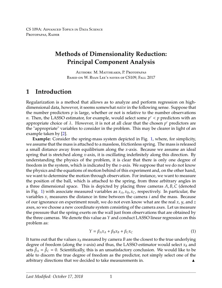
CS 109A: A dvanced T opics in D ata S cience P rotopapas , R ader Methods of Dimensionality Reduction: Principal Component Analysis A uthors : M. M attheakis , P. P rotopapas B ased on W. R yan L ee ’ s notes of CS109, F all 2017 1 Introduction Regularization is a method that allows as to analyze and perform regression on high- dimensional data, however, it seems somewhat naive in the following sense. Suppose that the number predictors p is large, whether or not is relative to the number observations n . Then, the LASSO estimator, for example, would select some p ′ < p predictors with an appropriate choice of λ . However, it is not at all clear that the chosen p ′ predictors are the "appropriate" variables to consider in the problem. This may be clearer in light of an example taken by [2]. Example: Consider the spring-mass system depicted in Fig. 1, where, for simplicity, we assume that the mass is attached to a massless, frictionless spring. The mass is released a small distance away from equilibrium along the x -axis. Because we assume an ideal spring that is stretched along x -axis, it is oscillating indefinitely along this direction. By understanding the physics of the problem, it is clear that there is only one degree of freedom in the system, which is indicated by the x -axis. We suppose that we do not know the physics and the equations of motion behind of this experiment and, on the other hand, we want to determine the motion through observation. For instance, we want to measure the position of the ball, which is attached to the spring, from three arbitrary angles in a three dimensional space. This is depicted by placing three cameras A , B , C (denoted in Fig. 1) with associate measured variables as x A , x B , x C , respectively. In particular, the variables x j measures the distance in time between the camera i and the mass. Because of our ignorance on experiment result, we do not even know what are the real x , y , and z axes, so we choose a new coordinate system consisting of the camera axes. Let us measure the pressure that the spring exerts on the wall just from observations that are obtained by the three cameras. We denote this value as Y and conduct LASSO linear regression on this problem as: Y = β A x A + β B x B + β C x C (1) It turns out that the values x B measured by camera B are the closest to the true underlying degree of freedom (along the x -axis) and thus, the LASSO estimator would select x B and sets ˆ β A = ˆ β C = 0. Scientifically, this is an unsatisfactory conclusion. We would like to be able to discern the true degree of freedom as the predictor, not simply select one of the arbitrary directions that we decided to take measurements in. � Last Modified: October 17, 2018 1
Figure 1: Toy example of an experiment on a spring system, taken from Shlens (2003). [2]. In a similar vein, when we examine a dataset with a number (or dimensions) of predictors p , we may suspect that the data actually lie on a lower-dimensional manifold. In the same sense, the three measurements of the previous example were necessary to situate the ball on a spring but the data had only one true degree of freedom. Thus, rather than variable selection methods such as LASSO, we may want to consider more sophisticated techniques for learning the intrinsic dimensionality of the data, a field known as dimensionality reduction or manifold learning . 2 Preliminaries in Linear Algebra and Statistics The above example and discussion serve to motivate the introduction of Principal Compo- nent Analysis (PCA). In this section we are giving a brief overview of linear algebra and statistics, which have been discussed in the first advanced section and are essential for the PCA foundation. 2.1 Linear Algebra R n × p . Along For this section, let X denote an arbitrary n × p matrix of real numbers, X ∈ I these notes we assume that the reader is familiar with the basic matrix computations that are discussed in the first advanced section, such as matrix multiplication, transpose, row reduction, and eigenvalue / eigenvector determination. For any such matrix X, the matrices X T X and XX T are symmetric. Proposition 1.1 Proof: To show symmetry of a matrix A it su ffi ces to show that A T = A . Clearly, this holds in our case, since T = X T ( X T ) T = X T X , ( X T X ) (2) and similarly for XX T . � Last Modified: October 17, 2018 2
The above proposition, while simple, is crucial due to an attractive property of real, symmetric matrices, as it is given in the following theorem. Indeed, the following is often considered as the fundamental theorem of linear algebra and known as the spectral theorem . Theorem 1.2 If A is a real, symmetric matrix, then there exists an orthonormal basis of eigenvectors of A. R m × m , we can find a basis { u 1 , ..., u m } such that the In order words, for any such matrix A ∈ I basis is orthonormal . That means that the basis vectors are orthogonal ( u i ⊥ u j so u T i u j = δ ij ) and normalized to unity ( || u i || 2 = 1). Moreover, this basis consists of eigenvectors of A , so that Au i = λ i u i for the eigenvalue λ i ∈ I R. Alternatively, if we stack the eigenvectors u i as rows we obtain the orthogonal matrix U T , where U T = U − 1 , and we can express the eigen-decomposition of A as A = U Λ U T , (3) where Λ = diag( λ i ) is the diagonal matrix of eigenvalues. The proof of the theorem is quite technical and we state the theorem here without proof. Moreover, there is a considerable amount of theory involving the set of eigenvalues of A , which is called its spectrum . The spectrum of a matrix reveals much about its properties, and although we do not delve into it here, we encourage the reader to refer to the bibliography for further details. We can, however, discuss one important property of the spectrum for the Gram matrices X T X and XX T ; namely, that the eigenvalues are non-negative as the following preposition states. The eigenvalues of X T X and XX T are non-negative reals. Proposition 1.3 Proof: Suppose λ is an eigenvalue of X T X with associated eigenvector u . Then, X T Xu = λ u u T X T Xu = u T λ u ( Xu ) T ( Xu ) = λ u T u || Xu || 2 = λ || u || 2 ⇒ λ > 0 (4) Since both || Xu || 2 and || u || 2 are non-negative, we conclude that λ > 0. Note that a zero eigenvalues is not acceptable because for λ = 0 the matrix X T X cannot be inverted. The result for XX T follows from a similar proof. � In fact, it turns out that the non-zero eigenvalues of these matrices are identical, as the following proposition shows. The matrices XX T and X T X share the same nonzero eigenvalues. Proposition 1.4 Proof: Suppose that λ is a non-zero eigenvalue of X T X with associated eigenvector u . Last Modified: October 17, 2018 3
Then X T Xu = λ u XX T Xu = X λ u XX T ( Xu ) = λ ( Xu ) XX T ˜ u = λ ˜ u (5) Thus, λ is an eigenvalue of XX T , with associated eigenvector ˜ u = Xu (rather than u ). � The trace of the gram matrix X T X is equal with the sum of its eigenvalues. Proposition 1.5 Proof: For the proof of the Proposition 1.5 , we first prove the cyclic property of the Trace, that is, we suppose an m × n matrix B and an n × n matrix C . Then, m m n � � � Tr ( BC ) = ( BC ) ii = B ij C ji i i j m n n � � � C ji B ij = ( CB ) jj = Tr ( CB ) , (6) i j j where we used the index notation for the trace and for the matrix multiplication. Knowing this property and by using the eigen-decomposition of Eq. (3), we prove Proposition 1.5 : Tr ( X T X ) = Tr ( U Λ U T ) = Tr ( U T U Λ ) = Tr ( Λ ) p � ⇒ Tr ( X T X ) = (7) , i = 1 note that the above property holds for any Gram matrix. λ i . � 2.2 Statistics R n × p as the model matrix. From this point on, In this section, we return considering X ∈ I we assume that the predictors are all centered , which means that for each column X j of X , we subtract the sample column mean n µ j = 1 � ˆ x ij , (8) n i = 1 so that we are considering the centered model matrix: � � ˜ X = X 1 − ˆ µ 1 , ..., X p − ˆ µ p . (9) Note that each column now has expectation zero, so that we can consider the sample covariance matrix : 1 X T ˜ ˜ S = X . (10) n − 1 Last Modified: October 17, 2018 4
Recommend
More recommend
Explore More Topics
Stay informed with curated content and fresh updates.
