[PPT] - Metabolic flux estimation So far in this course we have examined PowerPoint Presentation

SLIDE 1

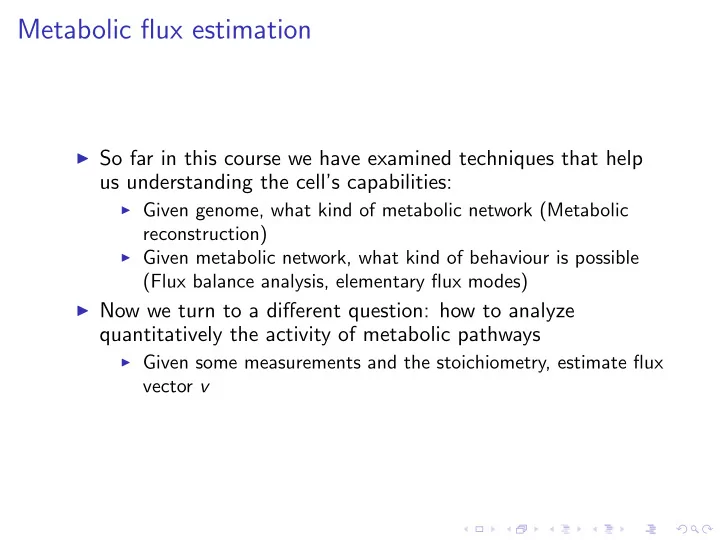
Metabolic flux estimation

◮ So far in this course we have examined techniques that help

us understanding the cell’s capabilities:

◮ Given genome, what kind of metabolic network (Metabolic

reconstruction)

◮ Given metabolic network, what kind of behaviour is possible

(Flux balance analysis, elementary flux modes)

◮ Now we turn to a different question: how to analyze

quantitatively the activity of metabolic pathways

◮ Given some measurements and the stoichiometry, estimate flux

vector v

SLIDE 2

The flux estimation problem

◮ In flux estimation the goal is to restrict the space of solutions

f the steady equations

Sv = 0

◮ Ideally, a single rate vector v is left as the solution ◮ In practise, we will need to resort to constraining the set of

solutions in the null space N(S).

SLIDE 3

The problem with alternative routes

◮ If there are alternative

routes to produce some metabolite in the metabolic network, the relative activity of the routes cannot be pinpointed.

◮ In the example on the

right, the fluxes vleft and vright cannot be pinpointed just by measuring exchange fluxes, only their sum can be solved.

◮ In this case the null space

f Sunknown is non-empty,

thus there is a choice of flux vectors that satisfy steady state

right v vleft vout vin vleft right v vout vin = = Material balance +

SLIDE 4

Isotope tracing experiments

◮ Isotope tracing experiments are the most accurate tool for

estimating the fluxes of alternative pathways

◮ In isotope tracing experiments the cell culture is fed a mixture

f natural and 13

C labeled substrate (e.g. 90%/10%).

◮ The fate of the 13

C labels is followed by measuring the intermediate metabolites by mass spectrometry or NMR

◮ From the enrichment of labels in the intermediates the fluxes

are inferred

SLIDE 5

13

C-Isotopomers

◮ In isotope tracing experiments the cell culture is fed a mixture

f natural and 13

C substrate (e.g. 90%/10%).

◮ This induces different kinds of 13

C labeling patterns, isotopomers (isotopic isomers):

NH2 C C H OOH H H H

12 12 12

C NH2 H H H H C

12C 13 12

OOH C NH2 C C H OOH H H H

12 12 13C

NH2 C C C H OOH H H H

13 12 12

NH2 NH2 C C C H OOH H H H

13 13 12

C C C H OOH H H H

13 12 13

Ala 000 Ala 001 Ala 100 Ala 101 Ala 010 Ala 110

SLIDE 6

Isotopomers and alternative pathways

◮ The vector of relative frequencies of the isotopomers

IAla = [P{000 Ala}, P{001 Ala}, . . . , P{111 Ala}] ∈ [0, 1]23, is called an isotopomer distribution

◮ Isotopomer distributions can give information about the fluxes

f alternative pathways if the pathways manipulate the carbon

chains of the metabolites differently

NH2 C C H OOH H H H

12 12 12

C NH2 H H H H C

12C 13 12

OOH C NH2 C C H OOH H H H

12 12 13C

NH2 C C C H OOH H H H

13 12 12

NH2 NH2 C C C H OOH H H H

13 13 12

C C C H OOH H H H

13 12 13

Ala 000 Ala 001 Ala 100 Ala 101 Ala 010 Ala 110

SLIDE 7

Isotopomeric balance equations

◮ The steady state condition

for free alanine implies:

vpw1 + vpw2 = vALA

◮ The steady state

assumption needs to hold for each isotopomer separately

◮ We can write balance

equations for each isotopomer:

SLIDE 8

Flux estimation from incomplete isotopomer data

In practice, we are faced with incomplete isotopomer data:

◮ Not all isotopomer distributions can be measured, due too

sensitivity issues of measuring equipment.

◮ Complete isotopomer distributions can only rerely be

measured:

◮ MS data groups isotopomers of the same weight:

aP(010 ALA) + bP(100 ALA) = d

◮ NMR measurements require 13

C in a specific position e.g. the middle carbon in alanine P(010 ALA)

x1y P(x1yALA) = d.

We start by tackling the first difficulty.

SLIDE 9

Fragment equivalence

◮ Two fragments F ⊆ M and F ′ ⊆ M′ are equivalent if the

fragment marginal distributions of the respective isotopomer distributions of M and M′ are equal, irrespectively of the fluxes of the metabolic network

◮ When does the fragment equivalence hold true?

C − C − C C − C C

M M’ F’ F

SLIDE 10

Fragment equivalence in general

◮ Assume fragments produced by alternative pathways travel

intact and similarly oriented (i.e. no permutation) starting from the common source fragment

◮ The isotopomer distribution of that fragment remain

equivalent to the source along the alternative pathways

C−C−C C−C−C C−C−C C−C−C ρ ρ

1 2

C−C−C C−C−C C−C C C−C−C ρ ρ ρ ρ

3 4 1 2

C−C−C ρ ρ

1 2

SLIDE 11

Equivalence classes

◮ The equivalance relation for fragments induces equivalence

classes of fragments to the metabolic networks

◮ The isotopomer distribution is the theoretically the same for

the whole equivalence class

5 7 2 6 C − C C − C − C 1 3 6 2 4 5 7 8 9 10 9 C − C C C C C − C 4 C − C − C 3 1 C − C − C 11

SLIDE 12

Balance equations for fragments

◮ Assume we have deduced

fragment marginals of ALA12 for both pathways

◮ Balance equations for the

fragment ALA12:

SLIDE 13

Flux estimation from incomplete isotopomer data

So far we have assumed that isotopomer distributions can either be completely measured or not at all. In practice, we are faced with incomplete isotopomer data:

◮ MS data: our PIDC software generally groups some

isotopomers together so we get data like

aP(010 ALA) + bP(100 ALA) = d

◮ NMR measurements require 13

C in a specific position e.g. the middle carbon in alanine

P(010 ALA)

x1y P(x1yALA) = d.

SLIDE 14

Isotopomer measurements as linear constraints

Complete isotopomer distribution, NMR and mass spectrometric data, and the absence of isotopomer information all can be expressed as a set of linear constraints to the isotopomer distribution. So we model the measurements as sets of equations aTIALA =

xyz

axyzP{xyzALA} = d to the isotopomer distribution IALA, represented as a matrix system ATIALA = d

SLIDE 15

Vector space interpretation

◮ An n-carbon metabolite M is associated with a 2n-dimensional

isotopomer vector space IM, that has a coordinate axis for each isotopomer

◮ An isotopomer distribution

IAla = [P{000 Ala}, P{001 Ala}, . . . , P{111 Ala}] ∈ [0, 1]23, is a point in IAla and lies in the intersection of 8 hyperplanes of the form eT

xyzIAla = P{xyzALA} ◮ exyz is the unit vector along the coordinate axis of isotopomer xyzAla, i.e. e000 = (1, 0, 0, . . . , 0), e001 = (0, 1, 0, . . . , 0),

e111 = (0, . . . , 0, 1)

SLIDE 16

Fragment subspaces

◮ A n′-carbon fragment of a n-carbon metabolite defines a

2n′-dimensional subspace of the 2n-dimensional isotopomer space

◮ The fragment subspace is spanned by vectors that corresponds

to the fragment marginals of the isotopomer distribution, e.g. for Ala12 we have four basis vectors u00 = [e000 + e001]/ √ 2, u01 = [e010 + e011]/ √ 2, u10 = [e100 + e101]/ √ 2 and u11 = [e110 + e111]/ √ 2

◮ A fragment marginal of the isotopomer distribution is a point

in the subspace spanned by the above basis vectors, given as the intersection of hyperplanes uT

xyIAla = P{xyAla12}

which are collectively written as UTIAla = IAla12

SLIDE 17

Fragment marginal as an orthogonal projection

◮ The set of basis vectors u00, u01, u10, u11 is orthogonal: e.g.

2uT

00u01 = (e000 + e001)T(e010 + e011) =

= eT

000e010 + eT 000e011 + eT 001e010 + eT 001e011 = 0

(1) by the orthogonality of the unit vectors exyz

◮ The vectors have unit length ||uxy|| = 1 ◮ Thus the matrix

U = [u00u01u10u11] is orthonormal

◮ The matrix equation

UTIAla = IAla12 can be seen as the orthogonal projection of the original isotopomer distribution to the fragment subspace.

SLIDE 18

Mass spectrometric data

◮ In mass spectrometers, molecules with equal mass will reside

in a single peak

◮ Thus, mass spectrum will group isotopomers with the same

number of labels.

◮ Thus we will get data of the form

mT

0 IAla = eT 000IAla = d0

mT

1 IAla = (e001 + e010 + e100)TIAla = d1

mT

2 IAla = (e011 + e101 + e110)TIAla = d2

mT

3 IAla = (e111IAla = d3

which is called the mass isotopomer distribution

◮ The vectors m0, . . . , m3 are again an orthogonal set spanning

a ’measurement’ subspace of the isotopomer space

◮ The vector (d0, d1, d2, d3)T can be seen to be an orthogonal

projection of the (unknown) isotopomer distribution to the measurement subspace

SLIDE 19

Tandem mass spectrometry

◮ Tandem mass spectrometers fragment the molecule to be

measured.

◮ Thus one can measure the mass isotopomer distribution of

fragments in addition to that of the whole molecule m′T

0 IAla12 = uT 00IAla12 = d0

m′T

1 IAla12 = (u01 + u10)TIAla12 = d1

m′T

2 IAla12 = uT 11IAla12 = d2 ◮ Typically, (at least some of) the vectors m′ i are linearly

independent from the vectors mi. Thus they constrain the isotopomer distribution more than the ’vanilla’ MS spectrum would

SLIDE 20

NMR measurements

◮ NMR measurements require 13

C in a specific position e.g. the middle carbon in alanine

◮ The form of the data is normalized abundances of such

specific isotopomers

P(010 ALA)

x1y P(x1yALA) = d.

◮ The data can be represented in the isotopomer space:

P(010 ALA) = d

x1y

P(x1yALA) nTIAla = (d, . . . , d − 1, . . . , d)TIAla = 0

◮ Thus, NMR data also introduced linear constraints to the

isotopomer distribution

SLIDE 21

Measurements in general

◮ So we can model the

measurements as sets of equations aTIALA =

xyz

axyzP{xyzALA} = d to the isotopomer distribution IALA, represented as a matrix system ATIALA = d

◮ If matrix A is orthonormal,

the interpretation is an

rthogonal projection of

the isotopomer distribution to the measurement subspace

feasible isotopomer distributions

vector space S

SLIDE 22

Mapping measurement data to metabolite fragments

◮ Our goal is to propagate the measurement data within the

equivalance set of the fragments

◮ However, in general, the measurements are made for

metabolites not their fragments, so some translation is needed.

◮ For example, suppose we have the following measurement

from NMR: P(010 ALA)

x1y P(x1yALA) = d1,

P(011 ALA)

x1y P(x1yALA) = d2,

P(110 ALA)

x1y P(x1yALA) = d3,

P(111 ALA)

x1y P(x1yALA) = d4

SLIDE 23

Mapping measurement data to metabolite fragments

◮ For Ala12 we get the following isotopomer constraints:

P(01 Ala12)

x1 P(x1

Ala12) = P(010 Ala) + P(011 Ala)

x1y P(x1yAla)

= d1 + d2, P(11 Ala12)

x1 P(x1

Ala12) = P(110 Ala) + P(111 Ala)

x1y P(x1yAla)

= d3 + d4

◮ What is the general approach, assuming arbitrary linear

equation set as the measurement?

SLIDE 24

Mapping measurements to fragments

◮ All fragment distributions

lie within a subspace of the isotopomer space of the metabolite

◮ Measurements lie in

another subspace, the measurement space.

◮ What is common between

the measurement and the fragment can be expressed in terms of the intersection space

Intersection space Measurement space S Isotopomer space

f fragment F

SLIDE 25

Mapping measurements to fragments

◮ What is known about the

underlying isotopomer distribution is its projection to the measurement space

◮ The fragment marginal

distribution is a projection to the fragment subspace

◮ The projection to the

intersection space represented what is known about the fragment marginal based on the measurement

Intersection space measurement (unknown) isotopomer distribution Measurement space S Isotopomer space

f fragment F

SLIDE 26

Mapping measurements to fragments

◮ The uncertainty about the

isotopomer distribution translates to uncertainty about the fragment distributions

◮ The smaller the dimension

f the intersection space,

the less is known about the fragment

Intersection space

measurement (unknown) isotopomer distribution Measurement space S Isotopomer space

f fragment F

SLIDE 27

Mapping measurements to fragments

◮ The measurement

completely determines the fragment marginal if and

nly if the fragment

subspace is a subspace of the measurement space

◮ Both computing the

intersection space and the projections to it can be written in terms of linear algebra

Intersection space

measurement (unknown) isotopomer distribution Measurement space S Isotopomer space

f fragment F

SLIDE 28

Isotopomers of a product metabolite

◮ In the complete information case, we

could compute the isotopomer distribution

f a product from the distributions of the

fragments via P(xyzM3) = P(xyM1)P(zM2)

◮ In the case of incomplete information an

analogous procedure can be used, independently for each pair of isotopomer constraints of the reactants

C − C − C C − C C ρ

M F

xyz

cxyzP(xyzM3) =

xy

axyP(xyM1)

·
z

bzP(zM2)

,

where cxyz = axybz

SLIDE 29

Generalized isotopomer balances

Via the above described approach we can obtain isotopomer constraints for fluxes around a junction. Assume we have the follwing constraints ATIALA|pw1 = d1, ATIALA|pw2 = d2 and ATIALA = d. In a steady state get a generalized isotopomer balance d1 · vpw1 + d2 · vpw2 = d · vALA

SLIDE 30

General recipe for flux estimation

◮ Compute equivalence sets of fragments for the metabolic

network

◮ Project the isotopomer measurements of the metabolites to

the fragments

◮ Propagate the obtained isotopomer constraints accross the

equivalence classes

◮ Form balance equations for fragments at the boundaries of the

equivalence classes

◮ Solve the resulting linear equation system

SLIDE 31

Identifiability of the fluxes

The success of the flux estimation approach depends heavily on the amount of isotopomer measurements taken from the metabolism.

5 10 15 20 25 30 35 20 40 60 80 100 120 140 160 180 200

Propagation efficiency, 1000 repeats / # of measured metabolites

# of measured metabolites mean # of carbons having isotopomer information with flow analysis without flow analysis

SLIDE 32

Incompleteness of the linear approach

◮ The preceding approach for flux estimation works in the linear

framework

◮ We propagate isotopomer constraints accross the equivalence

classes in order to compute balance equations that are linear in the fluxes

◮ However, given incomplete isotopomer measurements one can

find situations where a non-linear balance equation can be written while a linear cannot.

SLIDE 33

Non-linear example

◮ Consider situation where

we want to estimate I3 given I11, I12, I21 and I22 with no measurement from the intermediate metabolites

◮ The carbons above the

junctions are not equivalent with carbons below the junctions, so it is not possible to estimate I3 independently from the fluxes

◮ The example contains four

elementary flux modes, corresponding to four different combinations of source carbons to the two-carbon target

I11 I12 I21 I22 I3 I1 I2 v12 v22 v21 v11 C C C C C C C C

SLIDE 34

Non-linear example

◮ We can draw and

equivalent example consisting of the four elementary flux modes

◮ A balance equation that is

quadratic in the fluxes can be written:

I11 I21 I22 I3 I12 C C C C C C v12 v22 v12 v21 v11 v22 v11 v21 v3

v3I3 = v11v21I11I21 + v11v22I11I22 + v12v21I12I21 + v12v22I12I22

SLIDE 35

Isotopomer systems in general

◮ The above example could be tackled by switching from linear

equation solver to a quadratic solver

◮ However, there is no principal limit to the degree of the

balance equation, so we are faced with a non-linear systems of arbitrary degree, if we want to utilize isotopomer information to the fullest

SLIDE 36

Iterative approach

An alternative approach to solving fluxes is based on iteratively solving the isotopomer system as follows:

1. Start with an initial guess of the flux vector v0
2. Compute a predicted isotopomer distributions ˜

I that should result, were the guess correct

3. Compare the predicted isotopomer distributions to the

measured ones ˆ I

4. If the distance
˜

I − ˆ I

is small enough, stop and return the

current guess flux vector

5. Otherwise, generate a new flux guess v and continue from

step 2.