Mesh-Free Applications for Static and Dynamically Changing Node - PowerPoint PPT Presentation
Mesh-Free Applications for Static and Dynamically Changing Node Configurations Natasha Flyer Computational Information Systems Lab National Center for Atmospheric Research Boulder, CO Meshes vs. Mesh-free discretizations Structured meshes:
Mesh-Free Applications for Static and Dynamically Changing Node Configurations Natasha Flyer Computational Information Systems Lab National Center for Atmospheric Research Boulder, CO
Meshes vs. Mesh-free discretizations Structured meshes: FD, DG, FV, Spectral Elements Requires domain decomposition / curvilinear mappings Unstructured meshes: FEM, DG, FV, Spectral Elements Improved geometric flexibility; requires triangles, tetrahedral, etc. Mesh-free: RBF-FD (Radial basis Func.-generated Finite Differences) Total geometric flexibility; needs node locations, but no connectivites, e.g. no triangles or mappings
General RBF-FD Concept Scattered data in 2D Collocate RBF, e.g. 2D Gaussians Find linear combination of RBF that fits all the data On a sphere In a 3D
Simplicity of f RB RBF-FD FD: Mes esh-Fr Free ee method Ex.: Stencil of n = 21 nodes z x 1 2 x n Get Gaussian matrix A , use Gaussian elimination to solve for weights !"#(−& ' (( ) !"#(−& ' (' ) . . . !"#(−& ' (+ ) . ( 0/0"[!"# −& ' ( ]| ⋮ ⋱ ⋮ ⋮ = ⋮ !"#(−& ' +( ) !"#(−& ' +' ) . . . . !"#(−& ' ++ ) . + 0/0"[!"# −& ' + ]|
Coding RBF-FD Method is FAST and EASY IDX = knnsearch(xyz,xyz,'K',n); % n is stencil size for k = 1:N % Loop over all points N in domain X = xyz(IDX(k,:),:); % nodes in the kth stencil r2 = (X(:,1) - X(:,1)').^2 + … (X(:,2) - X(:,2)').^2 + … (X(:,3) - X(:,3)').^2 ; % Distance matrix A = exp(-r2); % RBF-FD matrix RHS_dx = -2*(X(:,1) – X(k,1)).* exp(-r2); % derivative of GA w.r.t x,y,z RHS_dy = -2*(X(:,2) – X(k,2)).* exp(-r2); RHS_dz = -2*(X(:,3) – X(k,3)).* exp(-r2); Dx(k,:) = A\RHS_dx; % Differentiation matrices (DM) Dy(k,:) = A\RHS_dy; Dz(k,:) = A\RHS_dz; end Have DMs for any geometry and point distribution in 3D space
Translating Static Node Refinement (Flyer and Lehto, 2010, JCP ) !ℎ/!$ = &(( )*$. , )-./. , $) 1 2ℎ http://web.maths.unsw.edu.au/~rsw/Sphere/
Comparison between ME, MD, Refined, and other methods Method N D t (mins.) RMS error RBF, refined 900 60 5e-3 RBF, ME 3136 60 4e-3 RBF, MD 3136 60 5e-3 DG 9600 6 7e-3 FV 38,400 30 2e-3 FV, AMR 2500 to 165K Variable 2e-3
How we Cluster Nodes and Variable Shape Parameter Fine features in flow are formed where ! is large use ! to assign charge distribution for node repel ∝ sech + "#$. tanh "#$. = [0.1 + 0 * ! "#$. ] - 1 / "#$. ! "#$. When clustering nodes, the shape parameter of the Gaussian Exp[-( e r ) 2 ] must scale over the domain to avoid ill-conditioned matrices and Runge phenomena Rule-of-Thumb: e ∝ Inverse of Euclidean distance to nearest neighbor 2 / "#$. ! "#$. Node distribution 2 ! "#$.
Effect of Clustering on Error c = 1 c = 100 c = 0.1 c = 10 RMS Error, N = 1849
Dynamic Node Refinement: Simple Tropical Cyclogenesis (in collaboration with Erik Lehto) Barotropic Vorticity Equation = streamfunction = relative vorticity - We do not know apriori where fine features will occur - Need a good Monitor Function for node adaptation - Generally, takes the form ! = !($%) , % is a physical feature of the flow a is a scaling parameter ! ', ), * =
Steps in implementation 1. ! at a given time is approximated with RBFs 2. Assign charge distribution according 1/ ! and repel 3. Evaluate solution at new pts. via RBF interpolation Calculate spatially variable e and recalculate RBF differentiation matrices 4. 3500km x 3500km Separation Dist: 400km
3500km x 3500km Separation Dist: 410km
Coupled Reaction-diffusion equations over irregular surfaces (Pi Piret, , JCP 2012) The Brusselator equations (Alan Turning) model pattern formation in nature, Solved by RBF over the surface of a frog Snapshots from a computed time evolution for two different parameter regimes Tabasara rain frog Poison dart frog - RBF Node layout - AIM@Shape Online Repository
Movie Courtesy of Grady Wright
Node generation algorithms Iterative-Type Schemes Advancing-Front Type Schemes For a given number of nodes, For a given number of nodes, the quality of the distribution Start at a boundary and advance depends on how soon forward until the domain is filled. the iteration is stopped. - Dithering for half-tone images - Min. energy distribution - Voronoi relaxation Notice nice hex pattern. - Delaunay triangulations Instead of changing width of dots, we change density • DistMesh (Persson-Strang) of dots. We start at bottom • Gmsh (Geuzaine-Remacle) boundary and march upward until domain is filled Half-toneimage Human eye
Distributing variable node density on sphere (Fornberg and Flyer, 2015) Below: Gray scale rendering of the file topo.mat in Matlab’s Mapping toolbox Top right: Advanicng Front Algorithm N = 105,419 nodes rendering of the topo map above Computational speed in MATLAB still around 11,000 nodes per second. Next step in modeling (Bayona et al. 2015) : Take elevation physically taken into account
3D Elliptic PDE: Modeling Electrical Currents in the Atmosphere ( s ( x,y,z ) u ) = S(x,y,z) Thunderstorm sources 3D Node Layout Conductivity Elec. potential (NASA measured data) Topography to 8km 8 km Nested spherical shells 8km to 52km 52 km
Sparsity pattern of 3D elliptic operator (99.998% zeros) 3D node layout Nested Shell Nicely banded but GMRES CRASHES After using reverse Cuthill- McKee Before any node reordering Result: Testing with data, 4.2M nodes 100 km. lat. – long. By 600m vertical, 31 mins on laptop using GMRES GitHub Open Source Code: Bayona et al. , A 3-D RBF-FD solver for modelling the atmospheric Global Electric Circuit with topography (GEC-RBFFD v1.0), Geosci. Model Dev. 2015.
2D Compressible Navier-Stokes with Topography using RBF-FD Schematic node layout
Movie Courtesy of Gregory A. Barnett Simulation of a cold downdraught in a dry atmosphere at 300K
Recent Review Material for RBF 1. N. Flyer, G.B. Wright, and B. Fornberg, 2014. Radial basis function-generated finite differences: A mesh-free method for computational geosciences , Handbook of Geomathematics, Springer-Verlag 2. B. Fornberg and N. Flyer, 2015 Solving PDEs with Radial Basis Functions , Acta Numerica. 3. B. Fornberg and N. Flyer, 2015 A Primer on Radial Basis Functions with Applications to the Geosciences , SIAM Press .
Recommend
More recommend
Explore More Topics
Stay informed with curated content and fresh updates.
