Measuring the Cosmic Microwave Background with the South Pole - PowerPoint PPT Presentation
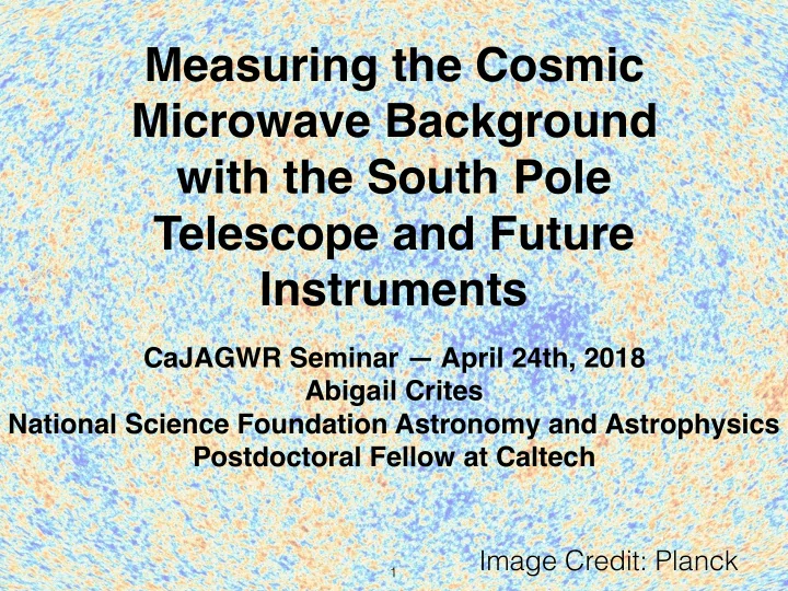
Measuring the Cosmic Microwave Background with the South Pole Telescope and Future Instruments CaJAGWR Seminar April 24th, 2018 Abigail Crites National Science Foundation Astronomy and Astrophysics Postdoctoral Fellow at Caltech Image
Measuring the Cosmic Microwave Background with the South Pole Telescope and Future Instruments CaJAGWR Seminar — April 24th, 2018 Abigail Crites National Science Foundation Astronomy and Astrophysics Postdoctoral Fellow at Caltech Image Credit: Planck 1
Objective: detect signatures from inflationary gravitational waves in the cosmic microwave background (CMB) probe physics of the universe fractions of a second after the big bang
Slide Credit: https://lisa.nasa.gov/ 3
The Cosmic Microwave Background Image Credit: Planck 4
Observing the Early Universe: (what makes it challenging) 1. The signals we are trying to measure are very tiny. 2. The wavelength of the light is different than what we measure with our eyes and every day cameras. (typical wavelengths = 1 - 3 mm) (and what makes it worthwhile) 1. We can probe physics when the universe was less complicated. 2. We can probe high energy physics that is hard to create in the modern universe.
CMB Instruments QUAD COBE Boomerang WMAP SPIDER PLANCK The South Pole Telescope: ACT SPT-SZ ACTpol BICEP SPTpol AdvACT BICEP 2 SPT-3G Keck Keck Array BICEP 3 POLARBEAR BICEP Array Simons Array NOT A COMPLETE LIST Simons Observatory
What do you need for a successful CMB instrument? Observing Site — the atmosphere is one of the biggest sources of noise Sensitivity — how faint are the signals you can measure Resolution — what scale objects you can measure
What do you need for a successful CMB instrument? CMB Bands: 1 mm - 3 mm 300 GHz - 100 GHz Image Credit: Credit: IRAM, France
Photo Credit: Forest Banks 9
What do you need for a successful CMB instrument? Sensitivity — lots of detectors with very low noise that work at these frequencies Key Technology: Superconducting Transition Edge Sensor (TES) Bolometer
Key Technology: Superconducting Transition Edge Sensor (TES) Bolometer Photons Very Sensitive Thermometer Weak Thermal Link
Key Technology: Superconducting Transition Edge Sensor (TES) Bolometer Al and Ti TESs (Sensitive Thermometer) Photons Absorber Very Sensitive Thermometer Weak Thermal Link Silicon Nitride Support Legs 8 mm Image Credit: TIME Collab.
Key Technology: Superconducting Transition Edge Sensor (TES) Bolometer normal resistor Ohm’s Law V = I x R voltage = current x resistance superconductor Temperature (Kelvin)
Key Technology: Superconducting Transition Edge Sensor (TES) Bolometer normal resistor Ohm’s Law V = I x R voltage = current x resistance Electro-Thermal R Feedback: T I = V / R superconductor Temperature (Kelvin)
Key Technology: Superconducting Transition Edge Sensor (TES) Bolometer Very Sensitive Thermometer George et al. 2014, JLTP ! Image and figure Credit: TIME Collab., George et al 2014 15
“Lots of Detectors” 2010-2015 2015-2019 2020 — 2025 CMB Experiment II III IV Stage Number of TES ~1000’s ~ 10,000 ~500,000 Detectors
> 1 million 8 mm pixels pixel size = 4 um Transition Edge Sensor pixel size 1000 = 4 mm pixels
Cryogenics superconductor Temperature (Kelvin) 3He Sorption Refrigerator Image Credit: Bhatia et al. 2000
pixel size 1000 = 4 mm pixels 20
13
What do you need for a successful CMB instrument? Resolution — what scale objects you can measure 10 m primary mirror 1.5 m primary mirror Image Credit: SPT Image Credit: ESA
Planck 143 GHz 50 deg 2 23
South Pole 13x resolution Telescope 50x deeper 150 GHz 50 deg 2 24
Science Objectives 0. Constrain the Cosmological Parameters Describing our Universe “Lambda CDM Cosmology” • Will the universe expand forever, or will it collapse? • Is the universe dominated by exotic dark matter? • What is the shape of the universe? • How and when did the first galaxies form? • Is the expansion of the universe accelerating rather than decelerating? Credit: NASA WMAP
Science Objectives 0. Constrain the Cosmological Parameters Describing our Universe “Lambda CDM Cosmology” What are the parameters the CMB constrains? Atoms (Baryons) Dark Matter Dark Energy Hubble Constant Reionization Redshift Spectral Tilt Credit: NASA WMAP
https://wmap.gsfc.nasa.gov/resources/camb_tool/index.html
https://wmap.gsfc.nasa.gov/resources/camb_tool/index.html 28
https://wmap.gsfc.nasa.gov/resources/camb_tool/index.html 29
https://wmap.gsfc.nasa.gov/resources/camb_tool/index.html 30
Connection to LIGO measurements! https://wmap.gsfc.nasa.gov/resources/camb_tool/index.html 31
LIGO vs. CMB Measurements of the Hubble Constant, Ho Figure Credit: The Ligo Scientific Collaboration And The Virgo Collaboration, The 1m2h Collaboration, The Dark Energy Camera Gw-em Collaboration And The Des Collaboration, The Dlt40 Collaboration, The Las Cumbres Observatory Collaboration, The Vinrouge Collaboration, The Master Collaboration, Et Al.
Science Objectives 1. detect signatures from inflationary gravitational waves in the cosmic microwave background (CMB) probe physics of the universe fractions of a second after the big bang
Science Objectives 1. Why is the universe homogeneous? Why is the universe flat? Inflation?! inflation is as exponential expansion of the universe in the first fractions of a second after the big bang
Science Objectives 2. measure gravitational lensing of the CMB by matter in our universe Properties of neutrinos affect the structure in our universe! Image Credit: Stompor et al 2015 Image Credit: Planck
Understanding the Power Spectrum of the CMB If the sky looks like this The power spectrum looks like this: Power spectrum slides courtesy of Phil Korngut
Understanding the Power Spectrum of the CMB If the sky looks like this The power spectrum looks like this: Power on a Given Scale Scale (l) Power spectrum slides courtesy of Phil Korngut
Understanding the Power Spectrum of the CMB If the sky looks like this The power spectrum looks like this: Power on a Given Scale Scale (l) Power spectrum slides courtesy of Phil Korngut
Understanding the Power Spectrum of the CMB If the sky looks like this The power spectrum looks like this: Power on a Given Scale Scale (l) Power spectrum slides courtesy of Phil Korngut
The sky looks like this And the power spectrum looks like this! Power on a Given Scale Scale (l) Credit: Planck, wikipedia
What do you need for a successful CMB instrument? ability to detect the polarization of the CMB signal 41
CMB Polarization Thomson scattering generates linear polarization. Image Credit: Hu and Dodelson, 2001
The CMB polarization can be decomposed in to E- modes and B-modes E B Image Credit: Seljak and Zaldarriaga
The TT and EE spectra probe acoustic oscillations in the early Universe TT acoustic oscillations EE E-mode polarization patterns
The BB spectrum probes gravitational waves from inflation! TT acoustic oscillations EE EE B-mode polarization patterns BB IGW Inflationary Gravitational wave oscillations BB auto- and cross-frequency spectra between BICEP2/Keck Array (150 GHz) and Planck (217 and 353 GHz), BKP find a 95 % upper limit of r < 0.12. (A Joint Analysis of BICEP2/Keck Array and Planck Data)
Upper Limits on the Stochastic Gravitational- Wave Background from Advanced LIGO’s First Observing Run Figure Credit: LIGO Scientific and Virgo Collaborations, 2017 46
The amplitude of the gravity wave signal depends on the energy scale of inflation TT EE BB IGW r == Tensor-to- scalar r = 0.01, 0.6 × 10 16 GeV ratio BB auto- and cross-frequency spectra between BICEP2/Keck Array (150 GHz) and Planck (217 and 353 GHz), BKP find a 95 % upper limit of r < 0.12. (A Joint Analysis of BICEP2/Keck Array and Planck Data)
Gravitational lensing of the CMB creates a BB signal at small angular scales TT EE lensing of EE to BB BB IGW r = 0.01 BB lensing
Neutrino mass affects lensing – CMB can measure ∑ m ν TT EE ∑ m ν = 0 BB IGW ∑ m ν = 1.5 eV BB lensing
CMB P olarization B-Mode Lensing Power Spectrum and Neutrino Mass • direct implication of massive neutrinos is a non-zero hot dark matter (HDM) • this suppresses the power spectrum due to neutrinos free streaming below the matter- radiation equality scale Image Credit: Abazajian et al, 2014 50
How do we make this measurement in practice?
South Pole Telescope 150 GHz 50 deg 2 52
Time Ordered Data to Maps Outline of a CMB map making pipeline 1. Read in raw data 2. Interpolate over short pointing glitches and timestream dropouts 3. cut on elnod response, both pixels partners being live, pointing and flagged bolometers (squid off, zero bias, etc). 4. Process data: relative calibration, polynomial subtraction 5. Time stream rms cut (removes very noisy timestreams), other cuts (glitchy timestreams. 6. Make left and right going scan maps 7. Make sum and difference maps for each observation 6. Make cuts of noisy maps 8. Coadd maps in to bundles of ~20 maps
Raw Data Image Credit: https://pole.uchicago.edu/blog/
Recommend
More recommend
Explore More Topics
Stay informed with curated content and fresh updates.
