MDL-Based Unsupervised Attribute Ranking Zdravko Markov Computer - PowerPoint PPT Presentation
MDL-Based Unsupervised Attribute Ranking Zdravko Markov Computer Science Department Central Connecticut State University New Britain, CT 06050, USA http://www.cs.ccsu.edu/~markov/ markovz@ccsu.edu MDL-Based Unsupervised Attribute Ranking
MDL-Based Unsupervised Attribute Ranking Zdravko Markov Computer Science Department Central Connecticut State University New Britain, CT 06050, USA http://www.cs.ccsu.edu/~markov/ markovz@ccsu.edu
MDL-Based Unsupervised Attribute Ranking • Introduction (Attribute Selection) • MDL-based Clustering Model Evaluation • Illustrative Example (“play tennis” data) • Attribute Ranking Algorithm • Hierarchical Clustering Algortihm • Experimental Evaluation • Conclusion
Attribute Selection • Supervised / Unsupervised. Find the smallest set of attributes that – maximizes predictive accuracy – best uncovers interesting natural groupings (clusters) in data according to the chosen criterion • Subset Selection / Ranking (Weighting) m attribute sets for m – Computationally expensive: 2 attributes – Assumes that attributes are independent
Supervised Attribute Selection • Wrapper methods create prediction models and use the predictive accuracy of these models to measure the attribute relevance to the classification task. • Filter methods directly measure the ability of the attributes to determine the class labels using statistical correlation, information metrics, probabilistic or other methods. • There exist numerous methods in this setting due to the wide availability of model evaluation criteria in supervised learning.
Unsupervised Attribute Selection • Wrapper methods evaluate a subset of attributes by the quality of clustering obtained by using these attributes. • Filter methods explore classical statistical methods for dimensionality reduction, like PCA and maximum variance, information-based or entropy measures. • There exist very few methods in this setting generally because of the difficulty to evaluate clustering models.
Clustering Model Evaluation Chapter 4: Evaluating Clustering - MDL-Based Model and Feature Evaluation http://www.cs.ccsu.edu/~markov/ http://www.cs.ccsu.edu/~markov/dmw4.pdf http://www.cs.ccsu.edu/~markov/dmwdata.zip http://www.cs.ccsu.edu/~markov/DMWsoftware.zip
Clustering Model Evaluation • Consider each possible clustering as a hypothesis H that describes ( explains ) data D in terms of frequent patterns (regularities). • Compute the description length of the data L ( D ), the hypothesis L ( H ), and data given the hypothesis L ( D|H ). • L ( H ) and L ( D ) are the minimum number of bits needed to encode (or communicate) H and D respectively. • L ( D|H ) represents the number of bits needed to encode D if we know H . • If we know the pattern of H, no need to encode all its occurrences in D, rather we may encode only the pattern itself and the differences that identify each individual instance in D .
Minimum Description Length (MDL) and Information Compression • The more regularity in D the shorter description length L ( D|H ). • Need to balance L ( D|H ) with L ( H ), because the latter depends on the complexity of the pattern. Thus the best hypothesis should – minimize the sum L ( H ) +L ( D|H ) ( MDL principle ) – or maximize L ( D ) – L ( H ) – L ( D|H ) ( Information Compression )
Encoding MDL • Hypotheses and data are uniformly distributed and the probability of occurrence of an item out of n alternatives is 1/ n . • Minimum code length of the message that a particular item has occurred is − log 2 1 /n = log 2 n bits. • The number of bits needed to encode the choice of k items out of n possible items is n 1 − = log log 2 2 n k k
Encoding MDL (attribute-value) • Data D , instance X ∈ D , X is a set of m attribute values, | X | = m = U • - set of all attribute values in D, k = | T | T X ∈ X D • Cluster C i is defined by the set of all attribute values T i ⊆ T that occur in its members , C i = { X ∈ C i , X ⊆ T i } • Clustering H = { C 1 ,C 2 ,…,C n } is defined by { T 1 ,T 2 ,…,T n } , k i = | T i | k n ∑ = + = L ( C ) log log n L ( H ) L ( C ) i 2 2 i k = i 1 i k n ∑ = × i = L ( D | C ) C log L ( D | H ) L ( D i C | ) i i i 2 i m = i 1 n k k ∑ = = + + × i MDL ( H ) MDL ( C ) MDL ( C ) log log n C log i i 2 2 i 2 k m = i 1 i
Play Tennis Data ID outlook temp humidity windy play 1 sunny hot high false no 2 sunny hot high true no 3 overcast hot high false yes 4 rainy mild high false yes 5 rainy cool normal false yes 6 rainy cool normal true no 7 overcast cool normal true yes 8 sunny mild high false no 9 sunny cool normal false yes 10 rainy mild normal false yes 11 sunny mild normal true yes 12 overcast mild high true yes 13 overcast hot normal false yes 14 rainy mild high true no C 1 = {1, 2, 3, 4, 8, 12, 14} (humidity=high) C 2 = {5, 6, 7, 9, 10, 11, 13} (humidity=normal) T 1 = {outlook=sunny, outlook=overcast, outlook=rainy, temp=hot, temp=mild, humidity=high, windy=false, windy=true} T 2 = {outlook=sunny, outlook=overcast, outlook=rainy, temp=hot, temp=mild, temp=cool, humidity=normal, windy=false, windy=true}.
Clustering Play Tennis Data k k = + + × i MDL ( C ) log log n C log i 2 2 i 2 k m i k 1 = | T 1 | = 8, k 2 = | T 2 | = 9, k = 10, m = 4, n = 2 10 8 = + + × = MDL ( C ) log log 2 7 log 49 . 39 1 2 2 2 8 4 10 9 = + + × = MDL ( C ) log log 2 7 log 53 . 16 2 2 2 2 9 4 MDL ({ C 1 , C 2 }) = MDL (humidity) = 102.55 bits 1. MDL (temp) = 101.87 2. MDL (humidity) = 102.56 3. MDL (outlook) = 103.46 4. MDL (windy) = 106.33 � Best attribute is temp
MDL Ranker • Let A have values v 1 , v 2 ,…, v p • Clustering { C 1 ,C 2 ,…,C p }, where C i = { X | x i ∈ X } A = ∅ • Let V i • For each data instance X = { x 1 , x 2 ,…, x m } • For each attribute A • For each value x i A ∪ { x i } A = V i • V i ∑ = m = A k V • i j j 1 • Compute MDL ({ C 1 ,C 2 ,…,C p }) � Incremental (no need to store instances) � Time O ( nm 2 ), n is the number of data instances � Space O ( pm 2 ), p is the max number of attribute values � Evaluates 3204 instances with 13195 attributes (trec data) in 3 minutes.
Experimental Evaluation Data Data Set Instances Attributes Classes reuters 1504 2887 13 reuters-3class 1146 2887 3 reuters-2class 927 2887 2 trec 3204 13195 6 soybean 683 36 19 soybean-small 47 36 4 iris 150 5 3 ionosphere 351 35 2 Java implementations of MDL ranking and clustering available from http://www.cs.ccsu.edu/~markov/DMWsoftware.zip
Experimental Evaluation Metrics D 1 ∑ = × Average Precision r PrecisionA tRank(k) • k D = k 1 q ∈ 1 if a D k 1 ∑ = i q = r PrecisionA tRank(k) r i i k 0 otherwise = i 1 • Classes-to-clusters accuracy (“true” cluster membership) root [5, 9] temperature=hot [2, 2] outlook=sunny [2] no outlook=overcast [2] yes temperature=mild [4, 2] windy=FALSE [2, 1] yes windy=TRUE [2, 1] yes temperature=cool [3, 1] windy=FALSE [2] yes windy=TRUE [1, 1] no ----------------------------------------- Clusters (leaves): 6 Correctly classified instances: 11 (78%)
Average Precision of Attribute Ranking Data set | D q | InfoGain MDL Error Entropy reuters 15 0.3183 0.1435 0.0642 0.0030 reuters-3class 10 0.3948 0.1852 0.1257 0.0027 reuters-2class 7 0.5016 0.2438 0.1788 0.3073 trec 14 0.4890 0.2144 0.0637 0.0010 soybean 16 0.6265 0.5606 0.3871 0.4152 soybean-small 2 0.6428 0.3500 0.0913 0.1213 iris 1 1.0000 1.0000 1.0000 0.3333 ionosphere 9 0.6596 0.5041 0.2575 0.4252 D q – set of attributes selected by Wrapper Subset Evaluator with Naïve Bayes classifier. InfoGain – supervised attribute ranking using Information Gain Evaluator. Error – unsupervised ranking based on evaluating the quality of clustering by the sum of squared errors . Entropy – unsupervised ranking based on the reduction of the entropy in data when the attribute is removed (Dash and Liu 2000).
Classes-To-Clusters Accuracy With Reuters Data 60 MDL ranked 55 50 InfoGain ranked % Accuracy 45 EM 40 35 30 25 20 2887 2000 1000 500 300 200 100 50 30 20 10 5 3 2 1 75 70 MDL ranked 65 InfoGain ranked % Accuracy k-means 60 55 50 45 40 2887 2000 1000 500 300 200 100 50 30 20 10 5 3 2 1
Classes-To-Clusters Accuracy With Reuters-3class Data 75 70 65 60 55 EM 50 45 MDL ranked 40 35 InfoGain ranked 30 2886 2000 1000 500 300 200 100 50 30 20 10 5 3 2 1 75 70 MDL ranked 65 InfoGain ranked K-means 60 55 50 45 40 2886 2000 1000 500 300 200 100 50 30 20 10 5 3 2 1
Classes-To-Clusters Accuracy With Soybean Data 80 70 60 50 EM 40 30 20 MDL ranked 10 InfoGain ranked 0 36 30 20 10 5 3 2 1 60 50 40 k-means 30 20 MDL ranked 10 InfoGain ranked 0 36 30 20 10 5 3 2 1
Recommend
More recommend
Explore More Topics
Stay informed with curated content and fresh updates.
