Maxim Likhachev 1 Motion/Path Planning Uncertainty and Planning - PDF document

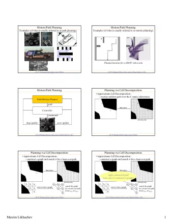
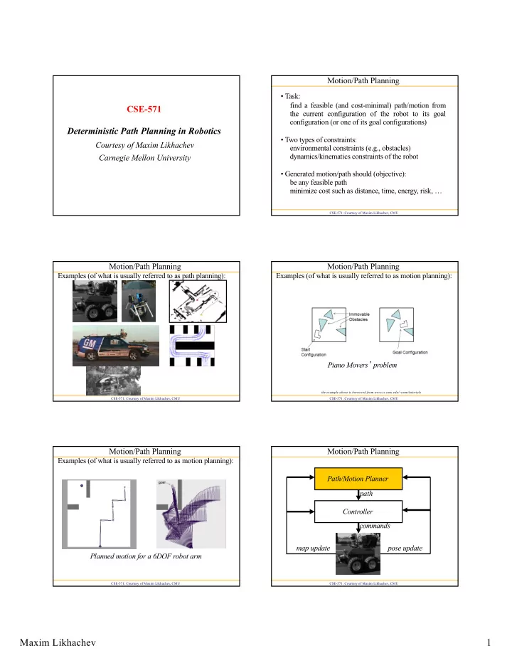
Motion/Path Planning • Task: find a feasible (and cost-minimal) path/motion from CSE-571 the current configuration of the robot to its goal configuration (or one of its goal configurations) Deterministic Path Planning in Robotics • Two types of constraints: Courtesy of Maxim Likhachev environmental constraints (e.g., obstacles) dynamics/kinematics constraints of the robot Carnegie Mellon University • Generated motion/path should (objective): be any feasible path minimize cost such as distance, time, energy, risk, … CSE-571: Courtesy of Maxim Likhachev, CMU Motion/Path Planning Motion/Path Planning Examples (of what is usually referred to as path planning): Examples (of what is usually referred to as motion planning): Piano Movers ’ problem the example above is borrowed from www.cs.cmu.edu/~awm/tutorials CSE-571: Courtesy of Maxim Likhachev, CMU CSE-571: Courtesy of Maxim Likhachev, CMU Motion/Path Planning Motion/Path Planning Examples (of what is usually referred to as motion planning): Path/Motion Planner path Controller commands map update pose update Planned motion for a 6DOF robot arm CSE-571: Courtesy of Maxim Likhachev, CMU CSE-571: Courtesy of Maxim Likhachev, CMU Maxim Likhachev 1

Motion/Path Planning Uncertainty and Planning • Uncertainty can be in: - prior environment (i.e., door is open or closed) Path/Motion Planner - execution (i.e., robot may slip) - sensing environment (i.e., seems like an obstacle but not sure) path - pose • Planning approaches: Controller - deterministic planning: - assume some (i.e., most likely) environment, execution, pose commands - plan a single least-cost trajectory under this assumption - re-plan as new information arrives map update pose update - planning under uncertainty: - associate probabilities with some elements or everything -plan a policy that dictates what to do for each outcome of sensing/action i.e., deterministic registration and minimizes expected cost-to-goal or Bayesian update i.e., Bayesian update (EKF) - re-plan if unaccounted events happen CSE-571: Courtesy of Maxim Likhachev, CMU CSE-571: Courtesy of Maxim Likhachev, CMU Uncertainty and Planning Uncertainty and Planning • Uncertainty can be in: • Uncertainty can be in: - prior environment (i.e., door is open or closed) - prior environment (i.e., door is open or closed) - execution (i.e., robot may slip) - execution (i.e., robot may slip) - sensing environment (i.e., seems like an obstacle but not sure) - sensing environment (i.e., seems like an obstacle but not sure) - pose - pose • Planning approaches: • Planning approaches: re-plan every time sensory data arrives or - deterministic planning: - deterministic planning: robot deviates off its path - assume some (i.e., most likely) environment, execution, pose - assume some (i.e., most likely) environment, execution, pose - plan a single least-cost trajectory under this assumption - plan a single least-cost trajectory under this assumption re-planning needs to be FAST - re-plan as new information arrives - re-plan as new information arrives - planning under uncertainty: - planning under uncertainty: - associate probabilities with some elements or everything - associate probabilities with some elements or everything -plan a policy that dictates what to do for each outcome of sensing/action -plan a policy that dictates what to do for each outcome of sensing/action and minimizes expected cost-to-goal and minimizes expected cost-to-goal - re-plan if unaccounted events happen computationally MUCH harder - re-plan if unaccounted events happen CSE-571: Courtesy of Maxim Likhachev, CMU CSE-571: Courtesy of Maxim Likhachev, CMU Example Control Architecture of Boss Urban Challenge Race, CMU team, planning with Anytime D* CSE-571: Courtesy of Maxim Likhachev, CMU CSE-571: Courtesy of Maxim Likhachev, CMU Maxim Likhachev 2

Trajectory Pre-Computation and Representing Motion Commands Optimization • State is position, curvature, and velocity < 𝑦,𝑧,𝜄,𝜆,𝑤 > • Velocity profiles determine forward speed Pre-compute parameters for set of end points < 𝑤 ) ,𝑤 . ,𝑤 - ,𝑏 ) ,𝑏 - ,𝑢 ) ,𝑢 - > • Spline represents shape and overall time < 𝜆 ) ,𝜆 * ,𝜆 + ,𝑡 - > Optimize (fine-tune) parameters initialized via interpolation CSE-571: Courtesy of Maxim Likhachev, CMU CSE-571: Courtesy of Maxim Likhachev, CMU Predicting and Avoiding Other Vehicles Passing and Cost CSE-571: Courtesy of Maxim Likhachev, CMU CSE-571: Courtesy of Maxim Likhachev, CMU Outline U-Turns • Deterministic planning - constructing a graph - search with A* - search with D* CSE-571: Courtesy of Maxim Likhachev, CMU CSE-571: Courtesy of Maxim Likhachev, CMU Maxim Likhachev 3

Outline Planning via Cell Decomposition • Approximate Cell Decomposition: • Deterministic planning - overlay uniform grid over the C-space (discretize) - constructing a graph - search with A* - search with D* discretize planning map CSE-571: Courtesy of Maxim Likhachev, CMU CSE-571: Courtesy of Maxim Likhachev, CMU Planning via Cell Decomposition Planning via Cell Decomposition • Approximate Cell Decomposition: • Approximate Cell Decomposition: - construct a graph and search it for a least-cost path - construct a graph and search it for a least-cost path discretize discretize eight-connected grid (one way to construct a graph) planning map planning map S 1 S 2 S 3 S 1 S 2 S 3 S 1 S 2 S 3 S 1 S 2 S 3 search the graph search the graph convert into a graph convert into a graph S 4 S 5 S 4 S 5 S 4 S 5 for a least-cost path S 4 S 5 for a least-cost path from s start to s goal from s start to s goal S 6 S 6 S 6 S 6 CSE-571: Courtesy of Maxim Likhachev, CMU CSE-571: Courtesy of Maxim Likhachev, CMU Planning via Cell Decomposition Planning via Cell Decomposition • Approximate Cell Decomposition: • Graph construction: - construct a graph and search it for a least-cost path - lattice graph - VERY popular due to its simplicity and representation of outcome state is the center of the corresponding cell arbitrary obstacles each transition is feasible - Problem: transitions difficult to execute on non-holonomic (constructed beforehand) robots action template replicate it discretize online CSE-571: Courtesy of Maxim Likhachev, CMU CSE-571: Courtesy of Maxim Likhachev, CMU Maxim Likhachev 4

Planning via Cell Decomposition Outline • Graph construction: • Deterministic planning - lattice graph - constructing a graph - pros: sparse graph, feasible paths - search with A* - cons: possible incompleteness - search with D* action template • Planning under uncertainty -Markov Decision Processes (MDP) -Partially Observable Decision Processes (POMDP) replicate it online CSE-571: Courtesy of Maxim Likhachev, CMU CSE-571: Courtesy of Maxim Likhachev, CMU A* Search A* Search • Computes optimal g-values for relevant states • Computes optimal g-values for relevant states at any point of time: at any point of time: an (under) estimate of the cost of a shortest path from s to s goal heuristic function g(s) g(s) the cost of a shortest path h(s) h(s) from s start to s found so far S S S 1 S 1 S start S start S goal S goal … … S 2 S 2 one popular heuristic function – Euclidean distance CSE-571: Courtesy of Maxim Likhachev, CMU CSE-571: Courtesy of Maxim Likhachev, CMU A* Search A* Search • Computes optimal g-values for relevant states • Computes optimal g-values for relevant states ComputePath function ComputePath function while( s goal is not expanded) while( s goal is not expanded) remove s with the smallest [f(s) = g(s)+h(s)] from OPEN ; remove s with the smallest [f(s) = g(s)+h(s)] from OPEN ; insert s into CLOSED ; insert s into CLOSED ; for every successor s ’ of s such that s ’ not in CLOSED for every successor s ’ of s such that s ’ not in CLOSED if g(s ’ ) > g(s) + c(s,s ’ ) if g(s ’ ) > g(s) + c(s,s ’ ) g(s 2 ) > g(s start ) + c(s start ,s 2 ) g(s ’ ) = g(s) + c(s,s ’ ); g(s ’ ) = g(s) + c(s,s ’ ); insert s ’ into OPEN ; insert s ’ into OPEN ; g= ¥ g= ¥ g= ¥ g= ¥ h=2 h=1 h=2 h=1 2 2 g=0 g=0 S 2 g= ¥ S 2 g= ¥ S 1 S 1 1 2 1 2 h=3 h=3 h=0 h=0 CLOSED = {} CLOSED = {} S start S start 1 1 S goal S goal OPEN = {s start } OPEN = {s start } 1 1 next state to expand: s start next state to expand: s start 3 3 S 4 S 4 S 3 S 3 g= ¥ g= ¥ g= ¥ g= ¥ h=2 h=1 h=2 h=1 Maxim Likhachev, University of Pennsylvania Maxim Likhachev, University of Pennsylvania Maxim Likhachev 5