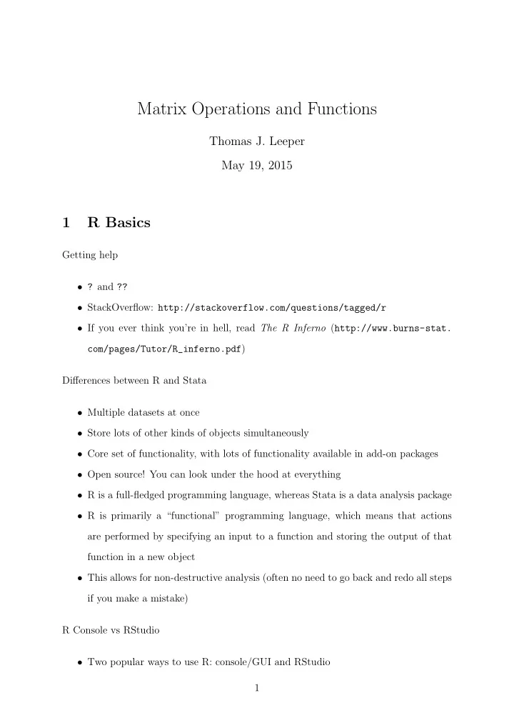
Matrix Operations and Functions Thomas J. Leeper May 19, 2015 1 R - PDF document

Matrix Operations and Functions Thomas J. Leeper May 19, 2015 1 R Basics Getting help • ? and ?? • StackOverflow: http://stackoverflow.com/questions/tagged/r • If you ever think you’re in hell, read The R Inferno ( http://www.burns-stat. com/pages/Tutor/R_inferno.pdf ) Differences between R and Stata • Multiple datasets at once • Store lots of other kinds of objects simultaneously • Core set of functionality, with lots of functionality available in add-on packages • Open source! You can look under the hood at everything • R is a full-fledged programming language, whereas Stata is a data analysis package • R is primarily a “functional” programming language, which means that actions are performed by specifying an input to a function and storing the output of that function in a new object • This allows for non-destructive analysis (often no need to go back and redo all steps if you make a mistake) R Console vs RStudio • Two popular ways to use R: console/GUI and RStudio 1

• R console or GUI is a basic interface • RStudio is an “integrated development environment” meant to make it easier to do some things • None of these have point and click menus • We’ll work in the console Basic operations of the console • Type commands and press enter (like in Stata) • Line continuation • Whitespace • Previous commands • Command completion • Clearing previous results • Limited menus • Objects, naming, classes x <- 1 x = 1 logical () integer () numeric () character () factor () class (1L) • basic math 2 + 2 1 - 3 4 * 5 6 / 3 2 ^ 2 # precedence 2 + 3 * 4 3 * 4 + 2 (2 + 3) * 4 2 + (3 * 4) • vectors 2

c(1,2,3) 1:3 c(1 ,3:4) c(TRUE , FALSE) c(1L, 2L) # missing values NA c(1,NA) c(NA ,TRUE) NULL c(1,NULL ,3) • coercion as.numeric(TRUE) as.integer(TRUE) as.logical (1) as.logical (-1) as.logical (3) as.integer (1.5) • logicals and boolean operations TRUE | TRUE TRUE | FALSE FALSE | FALSE TRUE & TRUE TRUE & FALSE FALSE & FALSE !TRUE !FALSE TRUE | 1L FALSE | 1L TRUE | 0L TRUE + TRUE TRUE - FALSE TRUE - (2* TRUE) # equality 1 == 1 1 == 1L TRUE == 1L 2 == 3 3

2 == TRUE 1 != 1 1 != 0 TRUE != 3 4 %in% 1:5 3:5 %in% c(2,4,6) !3:5 %in% c(2,4,6) • vector indexing (positional, logical, named) x <- letters x[1] x[2] x[1:3] x[c(1 ,3 ,5)] # seq seq_along(x) seq (1,5) # rep rep(1, 3) rep (1:2, times = 3) rep (1:2, each = 3) # indexing beyond range c(1 ,3 ,5)[2] c(1 ,3 ,5)[4] # negative indexing c(1 ,3 ,5)[ -1] # vectorized operations (1:3) + 1 # but remember precedence: 1:3 * 2 1:(3 * 2) 1:3[2] (1:3)[2] # recycling 1:4 + 1:2 1:3 + 1:2 # named indexing x <- 1:3 names(x) names(x) <- c(’one ’,’two ’,’three ’) names(x) x x[1] x[’one ’] x <- c(a = 1, b = 3, c = d) 4

x[’b’] • A data.frame is a collection of equal-length vectors. # built -in data.frames mtcars iris # data I/O install.packages(’rio ’) library(’rio ’) Questions? 2 Matrices and OLS Estimation If we have the following matrix:   − 1 3 (1)     2 − 4 We represent that in R as a vector of values passed to the matrix() function, which regulates the dimensions of the matrix: matrix(c(-1, 2, 3, -4), nrow = 2) # other examples matrix (1:6) matrix (1:6, nrow =2) matrix (1:6, ncol =3) matrix (1:6, nrow=2, ncol =3) matrix (1:6, nrow=2, ncol=3, byrow=TRUE) a <- matrix (1:10 , nrow =2) length(a) nrow(a) ncol(a) dim(a) rbind (1:3 ,4:6 ,7:9) cbind (1:3 ,4:6 ,7:9) # transpose t(rbind (1:3 ,4:6 ,7:9)) Manually calculate the transpose of a matrix! 5

Some special matrices: # identity matrix diag (3) # be careful with ‘diag ()‘. it does many different things # row vector matrix (1:5, nrow = 1) # column vector matrix (1:5, ncol = 1) Matrix indexing: b <- rbind (1:3 ,4:6 ,7:9) b[1,] #’ first row b[,1] #’ first column b[1,1] #’ element in first row and first column # vector (positional) indexing b[1:2 ,] b[1:2 ,2:3] # negative indexing b[ -1 ,2:3] # logical indexing b[c(TRUE ,TRUE ,FALSE ),] b[,c(TRUE ,FALSE ,TRUE )] # ‘diag ‘ for extraction diag(b) upper.tri(b) #’ upper triangle b[upper.tri(b)] lower.tri(b) #’ lower triangle b[lower.tri(b)] Matrix operations: # scalar addition/subtraction a <- matrix (1:6, nrow =2) a + 1 a - 1 a + 1:2 a - 1:2 # scalar multiplication/division a * 2 a / 2 a * 1:2 a / 1:2 # additivity property: (X + Y)’ = X’ + Y’ A <- matrix (1:6, nrow = 3) B <- matrix (7:12 , nrow = 3) 6

A + B t(A + B) t(A) + t(B) 2.1 OLS in matrix notation We start with a matrix representation of our regression equation: y = Xb + e We need to minimize the sum of squared residuals, e , so we flip our equation y = Xb + e to be e = y − Xb . This gives us the residuals from one estimation of our coefficients b . We don’t want to minimize the residuals, though, instead we want to minimize the sum of squared residuals. Conveniently, matrix notation is a very easy way of representing that because e is a vector and the sum of a squared vector is just the dot product (i.e., vector times itself; or a column vector times a row vector representation). S ( b ) = e ′ e = ( y − Xb ) ′ ( y − Xb ) = ( y ′ − b ′ X ′ )( y − Xb ) = y ′ y − y ′ Xb − b ′ X ′ y + b ′ X ′ Xb = y ′ y − 2 y ′ Xb + b ′ X ′ Xb Last step above is because b ′ X ′ y is 1x1, thus equal to its own transpose. How do we minimize an equation? To minimize, we set differentiate S ( b ), set to 0, and solve for b . 7

∂S ( b ) = 0 − 2 X ′ y + 2 X ′ Xb ∂b 0 = − 2 X ′ y + 2 X ′ Xb 2 X ′ y = 2 X ′ Xb X ′ y = X ′ Xb ( X ′ X ) − 1 X ′ y = b If we assume y is a linear function of Xb , then b is an unbiased estimator of β (i.e., E ( b ) = β ). Then variance of our coefficient estimates is: � ( X ′ X ) − 1 X ′ � � ( X ′ X ) − 1 X ′ � V ( b ) = V ( y ) � ( X ′ X ) − 1 X ′ � σ 2 I n � ( X ′ X ) − 1 X ′ � = = σ 2 ( X ′ X ) − 1 X ′ X ( X ′ X ) − 1 = σ 2 ( X ′ X ) − 1 Note assumptions of constant error variance. Other types of standard errors (e.g., clus- tered, heteroskedasticity-robust) would replace V ( y ) with something else. What do we need to know to be able to calculate this? • Creating a matrix to represent our data • Scalar multiplication • Matrix transpose • Matrix multiplication • Matrix inversion 8

• Matrix indexing in R and extraction of a matrix diagonal 2.2 Data as a design matrix A design matrix is 1 observation per row, one variable per column. In order to represent complex terms (power terms, interactions, transformations, indicator/dummy variables), we have to transform our original data.frame into a a purely numeric matrix, with no missing data, one column for each term in the model, and a column of 1’s to estimate the intercept. There can also be no linear dependence between columns. mtcars X <- as.matrix(mtcars[,c(’vs ’, ’am ’)]) X # interactions X[,1] * X[,2] X <- cbind(X, X[,1] * X[,2]) # power terms , etc. mtcars[,’mpg ’] ^ 2 # categorical variables mtcars [,"cyl"] mtcars [,"cyl"] == 4 mtcars [,"cyl"] == 6 mtcars [,"cyl"] == 8 as.numeric(mtcars [,"cyl"] == 4) model.matrix (~ 0 + factor(cyl), data = mtcars) # intercept! cbind(1, X) A major issue with constructing a design matrix is missingness. By default, Stata, R, and other packages will use available case analysis . We cannot have missing values if we want to calculate most statistics or, for example, estimate a regression model, so this is a reasonable approach but if we construct the design matrix manually, we also need to deal with missingness manually. # missing data NA x <- c(1,2,NA ,4) x 9

# simple , single imputation is.na(x) x[is.na(x)] x[is.na(x)] <- mean(x, na.rm = TRUE) # extracting complete cases d <- data.frame(a = 1:4, b = c(1,2,NA ,4), c = c(1,NA ,3 ,4)) complete.cases(d) d[complete.cases(d), ] 2.3 Matrix multiplication This is the dot product we saw earlier with vectors generalized to work for matrices. Matrices are conformable (i.e., can be multiplied) if they are m-by-n and n-by-p . So number of columns of the first matrix must match number of rows of the second matrix. Otherwise, non-conformable. The output matrix from matrix multiplication is an m-by-p matrix. # inner product (or dot product) of two vectors 1:3 %*% 2:4 1*2 + 2*3 + 3*4 # dot product only works for conformable vectors or matrices! 1:3 %*% 1:2 mm <- function(A,B){ m <- nrow(A) n <- ncol(B) C <- matrix(NA ,nrow=m,ncol=n) for(i in 1:m) { for(j in 1:n) { C[i,j] <- paste(’(’,A[i,],’*’,B[,j],’)’,sep=’’,collapse =’+’) } } print(C, quote=FALSE) } # conformability A <- matrix (1:6, nrow = 3) B <- matrix (2:5, nrow = 2) A %*% B B %*% A # non -conformable mm(A,B) # dimension of output A <- matrix (1:30 , ncol = 3) B <- matrix (1:3, nrow = 3) A %*% B mm(A,B) 10