Matrix Multiplication Example (Cost Analysis, 45 in 2.4) The Mundo - - PowerPoint PPT Presentation

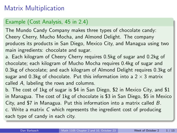
Matrix Multiplication

Example (Cost Analysis, 45 in 2.4)

The Mundo Candy Company makes three types of chocolate candy: Cheery Cherry, Mucho Mocha, and Almond Delight. The company produces its products in San Diego, Mexico City, and Managua using two main ingredients: chocolate and sugar.

• a. Each kilogram of Cheery Cherry requires 0.5kg of sugar and 0.2kg of

chocolate; each kilogram of Mucho Mocha requires 0.4kg of sugar and 0.3kg of chocolate; and each kilogram of Almond Delight requires 0.3kg of sugar and 0.3kg of chocolate. Put this information into a 2 × 3 matrix called A, labeling the rows and columns.

• b. The cost of 1kg of sugar is $4 in San Diego, $2 in Mexico City, and $1

in Managua. The cost of 1kg of chocolate is $3 in San Diego, $5 in Mexico City, and $7 in Managua. Put this information into a matrix called B.

• c. Write a matrix C which represents the ingredient cost of producing

each type of candy in each city.

Dan Barbasch Math 1105 Chapter 2 and 10, October 23 Week of October 2 1 / 13

EXERCISE

Exercise

How much does it cost to produce CC in Mexico City? What about the other cities? COST = (c of S) × (amt of S) + (c of C) × (amt of C) CC in MC: 2 × 0.5 + 5 × 0.2. How do we organize the calculation so we get all the answers at once?

Dan Barbasch Math 1105 Chapter 2 and 10, October 23 Week of October 2 2 / 13

ANSWER Multiplication of matrices: cS cC SD 4 3 MC 2 5 M 1 7 CC MM AD aS 0.5 0.4 0.3 aC 0.2 0.3 0.3 CC MM AD SD 4 · 0.5 + 3 · 0.2 4 · 0.4 + 3 · 0.3 4 · 0.3 + 3 · 0.3 MC 2 · 0.5 + 5 · 0.2 2 · 0.4 + 5 · 0.3 2 · 0.3 + 5 · 0.3 M 1 · 0.5 + 7 · 0.2 1 · 0.4 + 7 · 0.3 1 · 0.3 + 7 · 0.3

Dan Barbasch Math 1105 Chapter 2 and 10, October 23 Week of October 2 3 / 13

Transition Matrix, Illustration

EXPLAINING TRANSITION MATRICES USING THE WEATHER Suppose in a certain region on any given day, the chance of the weather changing depends only on what the weather was doing on the previous

• day. To keep things simple, we will say that the weather has two states -

either wet or dry. Let’s say that the probability of being dry on any day is conditional ONLY upon whether or not it was dry the day before. Specifically lets assume that the probability of being dry on any day, given it was dry on the previous n, is 0.3. Using standard conditional probability notation we can write that Pr(Dt|Dy) = 0.3. Since dry is the complement of wet, we can say that Pr(Wt|Dy) = 0.7. Further, suppose we assume that the probability of being wet today, given it was wet yesterday is 0.6. Thus we can similarly write that Pr(Wt|Wy) = 0.6 and Pr(Dt|Wy) = 0.4.

Dan Barbasch Math 1105 Chapter 2 and 10, October 23 Week of October 2 4 / 13

Questions

Given that it is WET today, what is the probability that it will be wet two days from now? The probability that it will be wet today is 0.2. What is the probability it will be wet two days from now? What is the transition matrix for 2, 3, . . . , n days from now?

Dan Barbasch Math 1105 Chapter 2 and 10, October 23 Week of October 2 5 / 13

State Diagram

The situation is illustrated in what is known as a state diagram.

Dan Barbasch Math 1105 Chapter 2 and 10, October 23 Week of October 2 6 / 13

Tree Diagram

We can also describe this with a tree diagram.

Dan Barbasch Math 1105 Chapter 2 and 10, October 23 Week of October 2 7 / 13

Transition Matrix, Formal Definition

Definition

• A square n × n matrix

   p11 . . . p1n . . . . . . . . . p1n . . . pnn    is called a Transition Matrix if the 0 ≤ pij ≤ 1 and the sums along rows add up to 1.

• An 1 × n matrix, also called an n−row vector
• v1

. . . vn

• is called a probability vector if 0 ≤ vi ≤ 1, and the sum of the coordinates

is 1.

Dan Barbasch Math 1105 Chapter 2 and 10, October 23 Week of October 2 8 / 13

M =    P(1 | 1) P(2 | 1) . . . P(n | 1) . . . . . . . . . . . . P(1 | n) P(2 | 1) . . . P(n | n)   

Definition (Markov Chain)

1 Finitely Many Outcomes. 2 Next State depends Only on Current State; gives rise to the matrix. 3 Always “The Same” (sketchy description, check the text). Dan Barbasch Math 1105 Chapter 2 and 10, October 23 Week of October 2 9 / 13

Example

M =   0.1 0.2 0.7 0.2 0.3 0.5 0.3 0.1 0.6   v =

• 0.3

0.3 0.4

• Dan Barbasch

Math 1105 Chapter 2 and 10, October 23 Week of October 2 10 / 13

Inverse Matrix

Definition

The Identity Matrix In×n is      1 . . . 1 . . . . . . . . . . . . . . . . . . 1     . It satisfies I · M = M and N · I = N for any M, N for which you can perform the multiplication. The inverse matrix to an n × n matrix A is a matrix B such that A · B = I. Alternatively B · A = I. If one holds, both hold. If the inverse exists, it is unique. The inverse is written B−1.

Dan Barbasch Math 1105 Chapter 2 and 10, October 23 Week of October 2 11 / 13

Example of Inverse

A =   1 2 2 1 3 1  . find its inverse if it exists.

Dan Barbasch Math 1105 Chapter 2 and 10, October 23 Week of October 2 12 / 13

Encoding

Encode the message To be or not to be. In numbers, 20, 15, 27, 2, 5, 27, 15, 18, 27, 14, 15, 20, 27, 20, 15, 27, 2, 5. A to Z are 1 to 26 and spaces are 27. You substitute, and break up into 3 × 1 column vectors. The encoded message is B · vi. To decode, you break up into groups of three and make column vectors. Then apply B−1.   2 4 6 −1 −4 −3 1 −1  .

Dan Barbasch Math 1105 Chapter 2 and 10, October 23 Week of October 2 13 / 13