Math 211 Math 211 Lecture #37 The Linearization in Higher - PDF document

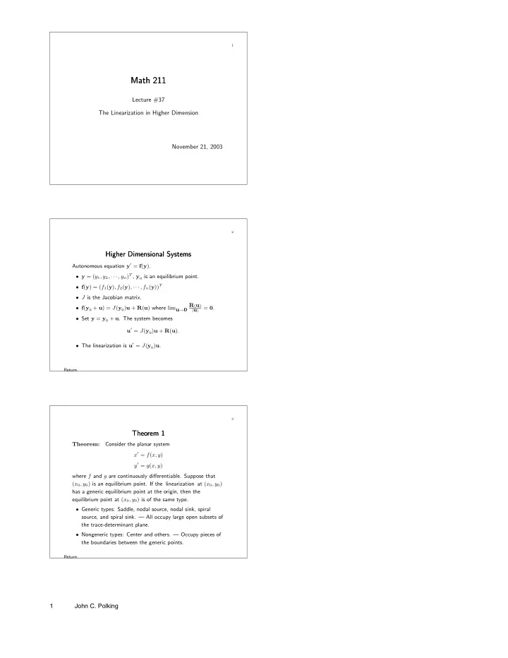
1 Math 211 Math 211 Lecture #37 The Linearization in Higher Dimension November 21, 2003 2 Higher Dimensional Systems Higher Dimensional Systems Autonomous equation y ′ = f ( y ) . • y = ( y 1 , y 2 , · · · , y n ) T , y 0 is an equilibrium point. • f ( y ) = ( f 1 ( y ) , f 2 ( y ) , · · · , f n ( y )) T • J is the Jacobian matrix. • f ( y 0 + u ) = J ( y 0 ) u + R ( u ) where lim u → 0 R ( u ) = 0 . | u | • Set y = y 0 + u . The system becomes u ′ = J ( y 0 ) u + R ( u ) . • The linearization is u ′ = J ( y 0 ) u . Return 3 Theorem 1 Theorem 1 Consider the planar system Theorem: x ′ = f ( x, y ) y ′ = g ( x, y ) where f and g are continuously differentiable. Suppose that ( x 0 , y 0 ) is an equilibrium point. If the linearization at ( x 0 , y 0 ) has a generic equilibrium point at the origin, then the equilibrium point at ( x 0 , y 0 ) is of the same type. • Generic types: Saddle, nodal source, nodal sink, spiral source, and spiral sink. — All occupy large open subsets of the trace-determinant plane. • Nongeneric types: Center and others. — Occupy pieces of the boundaries between the generic points. Return 1 John C. Polking

4 Theorem 2 Theorem 2 Suppose that y 0 is an equilibrium point for Theorem: y ′ = f ( y ) . Let J be the Jacobian of f at y 0 . 1. Suppose that the real part of every eigenvalue of J is negative. Then y 0 is an asymptotically stable equilibrium point. 2. Suppose that J has at least one eigenvalue with positive real part. Then y 0 is an unstable equilibrium point. Return Linearization Theorem 1 5 Example Example x ′ = − 2 x − 4 y + 2 xy y ′ = x − 6 y + x 2 − y 2 • The origin (0 , 0) is an equilibrium point. • The Jacobian has one eigenvalue, λ = − 4 , of algebraic multiplicity 2. • Theorem 1 does not apply. • Theorem 2 ⇒ the origin is a sink. Return 6 The Lorenz System The Lorenz System x ′ = − ax + ay y ′ = rx − y − xz z ′ = − bz + xy • Equilibrium points. � ( r ≤ 1 ) (0 , 0 , 0) � � ( r > 1 ) Set s = b ( r − 1) . The equilibrium points are (0 , 0 , 0) , and c ± = ( ± s, ± s, r − 1) . Return 2 John C. Polking

7 • The Jacobian is ⎛ ⎞ − a a 0 J = r − z − 1 − x ⎝ ⎠ y x − b � (0 , 0 , 0) ◮ If r < 1 (0 , 0 , 0) is asymptotically stable. ◮ If r > 1 (0 , 0 , 0) is unstable. Return 8 � c + and c − ◮ For 1 < r < 470 / 19 ≈ 24 . 74 , c + and c − are asymptotically stable. ◮ For r > 470 / 19 ≈ 24 . 74 , c + and c − are unstable. • As r varies the Lorenz system displays a wide variety of behaviors. � Use a = 10 and b = 8 / 3 . � For r = 100 there is a periodic attractor. � For r = 28 we have Lorenz’s strange attractor. � For r = 200 there is another strange attractor. c + & c − Return Jacobian 9 Invariant Sets Invariant Sets Definition: A set S is (positively) invariant for the system y ′ = f ( y ) if y (0) = y 0 ∈ S implies that y ( t ) ∈ S for all t ≥ 0 . • Examples: � An equilibrium point. � Any solution curve. Return 3 John C. Polking

10 Example — Competing Species Example — Competing Species x ′ = (5 − 2 x − y ) x y ′ = (7 − 2 x − 3 y ) y • The positive x - and y -axes are invariant. • The positive quadrant is invariant. � Populations should remain nonnegative. • The set S = { ( x, y ) | 0 < x < 3 , 0 < y < 3 } is positively invariant. Return 11 Nullclines Nullclines x ′ = f ( x, y ) y ′ = g ( x, y ) Definition: The x -nullcline is the set defined by f ( x, y ) = 0 . The y -nullcline is the set defined by g ( x, y ) = 0 . • Along the x -nullcline the vector field points up or down. • Along the y -nullcline the vector field points left or right. • The nullclines intersect at the equilibrium points. Return 12 Competing Species Competing Species x ′ = (5 − 2 x − y ) x y ′ = (7 − 2 x − 3 y ) y • x -nullcline: two lines x = 0 and 2 x + y = 5 . • y -nullcline: two lines y = 0 and 2 x + 3 y = 7 . • Two of the four regions in the positive quadrant defined by the nullclines are positively invariant. • This information allows us to predict that all solutions in the positive quadrant → (2 , 1) as t → ∞ . Return Nullclines 4 John C. Polking