Managerial Economics Ko University Graduate School of Business - PDF document
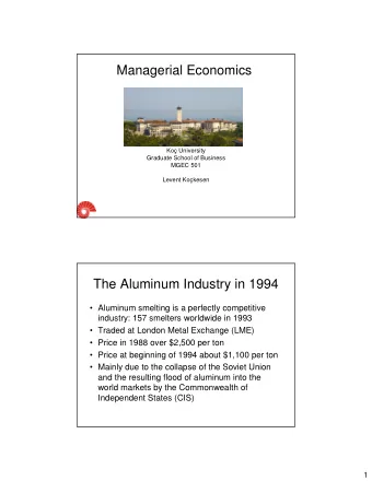
Managerial Economics Ko University Graduate School of Business MGEC 501 Levent Kokesen Perfectly Competitive Markets 1. What is Perfect Competition? 2. Supply Decision 3. Short-Run Equilibrium 4. Long-Run Equilibrium 1 Introduction
Managerial Economics Koç University Graduate School of Business MGEC 501 Levent Koçkesen Perfectly Competitive Markets 1. What is Perfect Competition? 2. Supply Decision 3. Short-Run Equilibrium 4. Long-Run Equilibrium 1
Introduction • Nakao Growers, Inc. is one of the largest of the 250 rose growers in the United States • It accounts for less than 5% of US production • Typical rose grower accounts for less than 1% • Its production decisions have no effect on the market price – key decision is how many rose stems to produce given the market price Why Study Perfect Competition? • Many other markets are approximately perfectly competitive, such as – most agricultural products – minerals and metals – oil tanker shipping • Tools and concepts that we will develop here will also be useful when we study other market structures – profit maximization – role of marginal revenue and marginal costs – entry/exit decisions 2
What is Perfect Competition? 1. uniform products: consumers regard them as identical The Law of One Price 2. buyers and sellers have perfect information about prices 3. buyers and sellers too small to Price Taking Behavior influence product and input prices 4. firms (existing and potential) Free Entry have equal access to resources Profit Maximization • What are “economic profits”? – Sales Revenue-Economic (opportunity) Cost • Example: You operate your own business Sales revenue $1M Cost of supplies $850K and labor Your best $200K outside offer Accounting profit = $1M – $850K = $150K Economic profit = $1M – $850K – $200K = –$50K 3
Profit Maximization • Owner is an investor who put his $500K down to start the business • Best return he could get alternatively is 12% - or $60K a year • Economic cost includes this return as opportunity cost of capital Economic profit = $1M – $850K – $60K = $90K Profit Maximization • Economic profit is given by π (Q) = TR(Q) – TC(Q) = PQ – TC(Q) • The firm chooses Q to maximize profits • Remember: MR > MC Produce more MR < MC Produce less MR = MC Optimal 4
Example ������������� ��� � ���������� � TC(Q) 1000 800 ������ TR(Q) 600 ����������� 400 200 π ����������� ��������� � � �������� � 0 0 10 20 30 40 50 -200 π π (Q) π π -400 75 ������������ ����������� � MC(Q) 60 ���������� 45 ������������� 30 MR(Q) 15 ��������� ����������� � 0 6 0 10 20 30 40 50 ���������������� Profit Maximization • Two conditions for profit maximization: P = MC(Q) MC is increasing • Is that it? • You have to check the endpoint Q = 0 • π (0) = 0 < π (30) 5
Supply Decision of a Firm P = MC(Q*) First order condition MC Second order condition π (Q*) ≥ π π (0) Produce Q* π π π π π π π (Q*) < π π (0) Produce 0 π π π π Short-Run Equilibrium Short-run: – there are fixed inputs (costs) – number of firms in the industry is fixed + + > SFC NSFC TVC(Q) , Q 0 = STC(Q) SFC , Q = 0 STC = short-run total costs SFC = sunk fixed costs – not avoidable even when Q = 0 NSFC = non-sunk fixed costs – can be avoided by setting Q = 0 TVC = total variable costs – non-sunk 6
Offshore Oil Rigs Offshore Oil Rigs There are numerous independent contractors hired by petroleum companies (e.g. Shell) to operate offshore oil rigs For a contractor quantity of output is the number of wells drilled within a particular period of time Variable Costs Fixed Costs Drilling Supplies Maintenance Fuel Food Medical Care Wages Insurance Which of the fixed costs are sunk depends on the period of time during which the rig will stay idle (i.e., produce zero output) 7
Offshore Oil Rigs Hot stacking: rig is taken out of service temporarily (perhaps for a few weeks), but remains fully staffed and ready on short notice to begin drilling again - all fixed costs are sunk Warm stacking: rig is taken out of service temporarily for a longer period of time (perhaps for a few months) - some maintenance and some labor costs are non-sunk Cold stacking: rig is taken out of service for a significant amount of time. The crew is laid off and the doors are welded shut. - only insurance costs are sunk Short-Run Supply when NSFC = 0 This implies TFC = SFC Profit maximization conditions: Given P supply is given by the following conditions 1. P = MC(Q) 2. MC increasing PQ – TVC(Q) – TFC > – TFC 3. π π (Q) > π π (0) π π π π PQ > TVC(Q) P > AVC(Q) 8
Price is P 1 P = MC Q = Q 1 MC increasing Price P > AVC(Q 1 ) S(P 1 ) = Q 1 SAC(Q) SMC(Q) Price is P 2 P 1 P = MC Q = Q 2 AVC(Q) MC increasing P > AVC(Q 2 ) S(P 2 ) = Q 2 P 2 Price is P 3 P S P 3 P = MC Q = Q 3 MC increasing P < AVC(Q 3 ) 0 Q 3 Q 2 Q 1 Q per period S(P 3 ) = 0 P S = shut-down price (min AVC) For any price below P S supply is zero Price SAC(Q) SMC(Q) S(P) AVC(Q) P S 0 Q per period 9
positive Price economic profits SAC(Q) SMC(Q) P 1 AVC(Q) P 2 negative economic profits 0 Q 2 Q 1 Q per period Example: Oil Rig Contractor STC(Q) = 8 + 0.25Q + 0.5Q 2 SFC = $ 8 mil SAC(Q) = 8/Q + 0.25 + 0.5Q NSFC = 0 AVC(Q) = 0.25 + 0.5Q TVC(Q) = 0.25Q + 0.5Q 2 SMC(Q) = 0.25 + Q 1. P = SMAC(Q) P = 0.25 + Q Q = P - 0.25 2. MC is always increasing 3. min AVC = 0.25 P S = 0.25 Price SMC(Q) − ≥ P 0 . 25 , if P 0 . 25 S ( P ) = 10.25 0 , if P < 0 . 25 To find min AC, set AC = MC and solve 0.25 + Q = 8/Q + 0.25 + 0.5Q SAC(Q) 0.5Q = 8/Q 6.05 Q 2 = 16 � Q = 4 AVC(Q) 4.25 min AC = 8/4 + 0.25 + 0.5x4 = 4.25 P = 10.25 SAC = 6.05 S = 10 0.25 profits = (10.25 – 6.05)10 = 42 4 10 Q per year 10
Short-Run Supply when NSFC > 0 TFC = SFC + NSFC Profit maximization conditions: Given P supply is given by the following conditions 1. P = MC(Q) 2. MC increasing PQ – TVC(Q) – TFC > – SFC 3. π π (Q) > π π π π π π (0) PQ > TVC(Q) + NSFC P > AVC(Q) + NSFC/Q average nonsunk cost (ANSC) Example: Oil Rig Contractor STC(Q) = 8 + 0.25Q + 0.5Q 2 SFC = $ 6 mil SAC(Q) = 8/Q + 0.25 + 0.5Q NSFC = $ 2 mil AVC(Q) = 0.25 + 0.5Q TVC(Q) = 0.25Q + 0.5Q 2 ANSC(Q) = 2/Q + 0.25 + 0.5Q min ANSC = 2.25 P S = 2.25 SMC(Q) = 0.25 + Q P − 0 . 25 , if P ≥ 2 . 25 = S ( P ) 0 , if P < 2 . 25 Price SMC(Q) To find min ANSC, set MC = ANSC and solve 0.25 + Q = 2/Q + 0.25 + 0.5Q SAC(Q) 0.5Q = 2/Q Q 2 = 4 � Q = 2 min AC = 2/2 + 0.25 + 0.5x2 = 2.25 ANSC(Q) AVC(Q) 2.25 0.25 Q per year 2 11
Price Price S S 2.25 0.25 2 Q per year Q per year Supply when all costs are sunk: Supply when some costs are nonsunk: if price is below $ 0.25 mil the oil rig is if price is expected to stay under $2.25 mil for a significant amount of time the rig is warm (or hot stacked cold) stacked. if price is expected to stay below $4.25 mil for a long period of time, the rig min SAC 4.25 should shut down and the contractor should leave the business Short-Run Market Supply Curve Number of firms is fixed: market supply is the sum of individual supplies P − 0 . 25 , if P ≥ 0 . 25 There are 100 of each type of firms S ( P ) = 1 0 , if P < 0 . 25 0 , < 0 . 25 − ≥ P P 0 . 50 , if P 0 . 50 = S ( P ) 2 − ≤ < 0 , if P < 0 . 50 100 ( P 0 . 25 ), 0 . 25 P 0 . 50 ( ) = S P This assumes that the input P − 0 . 75 , if P ≥ 0 . 75 100 ( 2 P − 0 . 75 ), 0 . 50 ≤ P < 0 . 75 S ( P ) = prices do not change as 3 0 , if < 0 . 75 P − ≥ 100 ( 3 P 1 . 50 ), P 0 . 75 market supply changes S 3 S 2 Price Price S 1 0.75 0.50 0.25 25 75 Q per year Q per year market supply 12
Short-Run Market Equilibrium Market Supply (100 identical firms) Typical oil rig contractor ( ) P − 0 . 25 , if P ≥ 0 . 25 100 P − 0 . 25 , if P ≥ 0 . 25 ( ) = ( ) = S P S P 0 , if P < 0 . 25 0 , if P < 0 . 25 Market Demand Market Equilibrium = − D ( P ) 825 100 P 825 − 100 P = 100 P − 25 = P 4 . 25 Q = 400 Price Price SMC(Q) S SAC(Q) AVC(Q) 4.25 D 0.25 4 Firm Q per year 400 Market Q per year Short-Run Market Equilibrium: Comparative Statics Initially the firms are making zero profits. But now suppose the market demand curve shifts up. The new demand function is given by ′ = − D ( P ) 975 100 P New market Equilibrium 975 − 100 P = 100 P − 25 = P 5 Q = 475 Price Price SMC(Q) positive economic profits S SAC(Q) 5 AVC(Q) D’ 4.25 D 0.25 4 4.75 Firm Q per year 400 475 Market Q per year 13
Recommend
More recommend
Explore More Topics
Stay informed with curated content and fresh updates.
