Machine Learning - MT 2017 4. Maximum Likelihood Varun Kanade - PowerPoint PPT Presentation

Machine Learning - MT 2017 4. Maximum Likelihood Varun Kanade University of Oxford October 16, 2017

Outline Probabilistic Perspective of Machine Learning ◮ Probabilistic Formulation of the Linear Model ◮ Maximum Likelihood Estimate ◮ Relation to the Least Squares Estimate 1

Outline Probability Review Linear Regression and Maximum Likelihood

Univariate Gaussian (Normal) Distribution The univariate normal distribution is defined by the following density function e − ( x − µ )2 1 X ∼ N ( µ, σ 2 ) √ p ( x ) = 2 σ 2 2 πσ Here µ is the mean and σ 2 is the variance. � ∞ p ( x ) d x = 1 −∞ � ∞ σ xp ( x ) d x = µ −∞ � ∞ Pr( a ≤ x ≤ b ) ( x − µ ) 2 p ( x ) d x = σ 2 a b Mean µ −∞ 2

Sampling from a Gaussian distribution Sampling from X ∼ N ( µ, σ 2 ) By setting Y = X − µ , sample from Y ∼ N (0 , 1) σ Cumulative distribution function � x 1 e − t 2 √ 2 dt Φ( x ; 0 , 1) = 2 π −∞ Φ( a ) a 1 1 Φ( a ) y ∼ Unif([0 , 1]) 0 0 a x 3

Bivariate Normal (Gaussian) Distribution Suppose X 1 ∼ N ( µ 1 , σ 2 1 ) and X 2 ∼ N ( µ 2 , σ 2 2 ) are independent The joint probability distribution p ( x 1 , x 2 ) is a bivariate normal distribution. p ( x 1 , x 2 ) = p ( x 1 ) · p ( x 2 ) � � � � − ( x − µ 1 ) 2 − ( x − µ 2 ) 2 1 1 √ √ = · exp · · exp 2 σ 2 2 σ 2 2 πσ 1 2 πσ 2 1 2  � � ( x − µ 1 ) 2 + ( x − µ 2 ) 2 1  −  = 2 ) 1 / 2 · exp 2 π ( σ 2 1 σ 2 2 σ 2 2 σ 2 1 2 � � 1 − 1 2 · ( x − µ ) T Σ − 1 ( x − µ ) = 2 π | Σ | 1 / 2 · exp where � � � � � � σ 2 0 µ 1 x 1 1 Σ = µ = x = σ 2 0 µ 2 x 2 2 Note: All equiprobable points lie on an ellipse. 4

Covariance and Correlation For random variable X and Y the covariance measures how the random variable change jointly � � cov( X, Y ) = E ( X − E [ X ]) · ( Y − E [ Y ]) Covariance depends on the scale. The (Pearson) correlation coefficient normalizes the covariance to give a value between − 1 and +1 . cov( X, Y ) corr( X, Y ) = � , var( X ) · var( Y ) where var( X ) = E [( X − E [ X ]) 2 ] and var( Y ) = E [( Y − E [ Y ]) 2 ] . Independent variables are uncorrelated, but the converse is not true! 5

Multivariate Gaussian Distribution Suppose x is a D -dimensional random vector. The covariance matrix consists of all pairwise covariances.   var( X 1 ) cov( X 1 , X 2 ) cov( X 1 , X D ) · · · cov( X 2 , X 1 ) var( X 2 ) cov( X 2 , X D )  · · ·  � ( x − E [ x ])( x − E [ x ]) T �   cov( x ) = E = . . . ... .   . . .  . . .    cov( X D , X 1 ) cov( X D , X 2 ) var( X D ) · · · If µ = E [ x ] and Σ = cov( x ) , the multivariate normal is defined by the density � � 1 − 1 2( x − µ ) T Σ − 1 ( x − µ ) N ( µ , Σ ) = (2 π ) D/ 2 | Σ | 1 / 2 exp 6

Suppose you are given three independent samples: x 1 = 0 . 3 , x 2 = 1 . 4 , and x 3 = 1 . 7 You know that the data is generated from either N (0 , 1) or N (2 , 1) . Let θ represent the parameters ( µ, σ ) of the two distributions. Then the probability of observing the data with parameter θ is called the likelihood. p ( x 1 , x 2 , x 3 | θ ) = p ( x 1 | θ ) · p ( x 2 | θ ) · p ( x 3 | θ ) We have to choose between θ = (0 , 1) or θ = (2 , 1) . Which one is more likely? x 1 x 2 x 3 µ = 0 µ = 2 Maximum Likelihood Estimation (MLE) Pick parameter θ that maximises the likelihood 7

Outline Probability Review Linear Regression and Maximum Likelihood

Linear Regression Linear Model y = w 0 x 0 + w 1 x 1 + · · · + w D x D + ǫ = w · x + ǫ Noise/uncertainty Model y given x , w as a random variable with mean w T x . E [ y | x , w ] = w T x We will be specific in choosing the distribution of y given x and w . Let us assume that given x , w , y is normal with mean w T x and variance σ 2 p ( y | w , x ) = N ( w T x , σ 2 ) = w T x + N (0 , σ 2 ) Alternatively, we may view this model as ǫ ∼ N (0 , σ 2 ) (Gaussian Noise) Discriminative Framework Throughout this lecture, think of the inputs x 1 , . . . , x N as fixed 8

Likelihood of Linear Regression (Gaussian Noise Model) Suppose we observe data � ( x i , y i ) � N i =1 . What is the likelihood of observing the data for model parameters w , σ ? MLE Estimator Find parameters which maximise the likelihood. (product of ‘‘likelihood density’’ segments) Least Square Estimator Find parameters which minimise the sum of squares of the residuals (sum of squares of the segments). 9

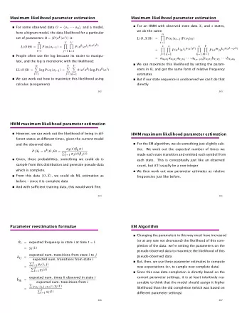
Likelihood of Linear Regression (Gaussian Noise Model) Suppose we observe data � ( x i , y i ) � N i =1 . What is the likelihood of observing the data for model parameters w , σ ? N � � � � � p y 1 , . . . , y N | x 1 , . . . , x N , w , σ = p y i | x i , w , σ i =1 According to the model y i ∼ w T x i + N (0 , σ 2 ) � � N � � � − ( y i − w T x i ) 2 1 √ p y 1 , . . . , y N | x 1 , . . . , x N , w , σ = 2 πσ 2 exp 2 σ 2 i =1   � � N/ 2 N � 1  − 1 ( y i − w T x i ) 2  = exp 2 σ 2 · 2 πσ 2 i =1 Want to find parameters w and σ that maximise the likelihood 10

Likelihood of Linear Regression (Gaussian Noise Model) Let us consider the likelihood p ( y | X , w , σ )   � � N/ 2 N � � � 1  − 1 ( y i − w T x i ) 2  p y 1 , . . . , y N | x 1 , . . . , x N , w , σ = exp 2 σ 2 · 2 πσ 2 i =1 As log : R + → R is an increasing function, we can instead maximise the log of the likelihood (called log-likelihood), which results in a simpler mathematical expression. N � LL( y 1 , . . . , y N | x 1 , . . . , x N , w , σ ) = − N 1 2 log(2 πσ 2 ) − ( y i − w T x i ) 2 2 σ 2 i =1 LL( y | X , w , σ ) = − N 1 2 log(2 πσ 2 ) − 2 σ 2 ( Xw − y ) T ( Xw − y ) In vector form, Let’s first find w that maximizes the log-likelihood 11

Maximum Likelihood and Least Squares Estimates We’d like to find w that maximises the log-likelihood 1 LL( y | X , w , σ ) = − N 2 log(2 πσ 2 ) − 2 σ 2 ( Xw − y ) T ( Xw − y ) Alternatively, we can minimise the negative log-likelihood 2 σ 2 ( Xw − y ) T ( Xw − y ) + N 1 2 log(2 πσ 2 ) NLL( y | X , w , σ ) = Recall the objective function we used for the least squares estimate in the previous lecture 1 2 N ( Xw − y ) T ( Xw − y ) L ( w ) = For minimizing with respect to w , the two objectives are the same upto a constant additive and multiplicative factor! 12

Maximum Likelihood Estimate for Linear Regression As the solution w ML to find the maximum likelihood estimator is the same as the least squares estimator, we have � � − 1 X T X X T y w ML = Recall the form of the negative log-likelihood 2 σ 2 ( Xw − y ) T ( Xw − y ) + N 1 2 log(2 πσ 2 ) NLL( y | X , w , σ ) = We can also find the maximum likelihood estimate for σ Exercise on sheet 2 to show that the MLE of σ is given by ML = 1 σ 2 N ( Xw ML − y ) T ( Xw ML − y ) 13

Prediction using the MLE for Linear Regression Given training data � ( x i , y i ) � N i =1 , we can obtain the MLE w ML and σ ML . One a new point x new , we can use these to make a prediction and also give confidence intervals y new = w ML · x new � y new + N (0 , σ 2 y new ∼ � ML ) 14

Summary : MLE for Linear Regression (Gaussian Noise) Model ◮ Linear model: y = w · x + ǫ ◮ Explicitly model ǫ ∼ N (0 , σ 2 ) Maximum Likelihood Estimation ◮ Every w , σ defines a probability distribution over observed data ◮ Pick w and σ that maximise the likelihood of observing the data Algorithm ◮ As in the previous lecture, we have closed form expressions ◮ Algorithm simply implements elementary matrix operations 15

Outliers and Laplace Distribution If the data has outliers, we can model the noise using a distribution that has heavier tails For the linear model y = w · x + ǫ , use ǫ ∼ Lap(0 , b ) , where the density function for Lap( µ, b ) is given by � � p ( x ) = 1 −| x − µ | 2 b exp b 0 . 3 1 0 . 2 0 . 5 0 . 1 0 0 − 3 − 2 − 1 0 1 2 3 − 6 − 4 − 2 0 2 4 6 Laplace and normal distributions with the same mean and variance 16

Maximum Likelihood for Laplace Noise Model Given data � ( x i , y i ) � N i =1 , let us express the likelihood of observing the data in terms model parameters w and b . � � N � −| y i − w T x i | 1 p ( y 1 , . . . , y N | x 1 , . . . , x N , w , b ) = 2 b exp b i =1   N � 1  − 1 | y i − w T x i |  = (2 b ) N exp b i =1 As in the case of the Gaussian noise model, we look at the negative log-likelihood N � NLL( y | X , w , b ) = 1 | y i − w T x i | + N log(2 b ) b i =1 Thus, the maximum likelihood estimate in this case can be obtained by minimising the sum of the absolute values of the residuals, which is the same objective we discussed in the last lecture in the context fitting a linear model that is robust to outliers. 17

Next Time ◮ Beyond Linearity: Basis Expansion, Kernels ◮ Regularization: Ridge Regression, LASSO ◮ Overfitting, Model Complexity, Cross Validation 18