Machine Learning for Signal Processing Independent Component - PowerPoint PPT Presentation

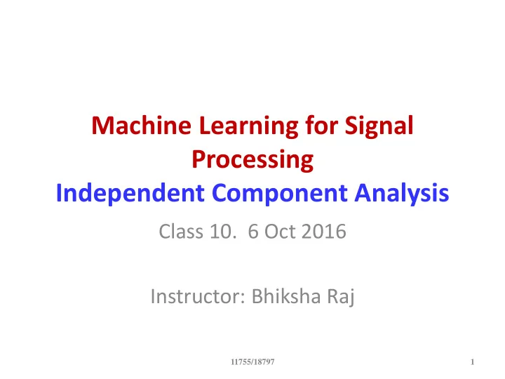
Machine Learning for Signal Processing Independent Component Analysis Class 10. 6 Oct 2016 Instructor: Bhiksha Raj 11755/18797 1

Revisiting the Covariance Matrix • Assuming centered data • C = S X XX T • = X 1 X 1 T + X 2 X 2 T + …. • Let us view C as a transform.. 11755/18797 2

Covariance matrix as a transform • ( X 1 X 1 T + X 2 X 2 T + … ) V = X 1 X 1 T V + X 2 X 2 T V + … • Consider a 2-vector example – In two dimensions for illustration 11755/18797 3

Covariance Matrix as a transform • Data comprises only 2 vectors.. • Major axis of component ellipses proportional to twice the length of the corresponding vector 4

Covariance Matrix as a transform Adding • Data comprises only 2 vectors.. • Major axis of component ellipses proportional to twice the length of the corresponding vector 5

Covariance Matrix as a transform Adding • More vectors.. • Major axis of component ellipses proportional to twice the length of the corresponding vector 11755/18797 6

Covariance Matrix as a transform Adding • More vectors.. • Major axis of component ellipses proportional to twice the length of the corresponding vector 11755/18797 7

Covariance Matrix as a transform • And still more vectors.. • Major axis of component ellipses proportional to twice the length of the corresponding vector 11755/18797 8

Covariance Matrix as a transform • The covariance matrix captures the directions of maximum variance • What does it tell us about trends? 11755/18797 9

Data Trends: Axis aligned covariance • Axis aligned covariance • At any X value, the average Y value of vectors is 0 – X cannot predict Y • At any Y, the average X of vectors is 0 – Y cannot predict X • The X and Y components are uncorrelated 11755/18797 10

Data Trends: Tilted covariance • Tilted covariance • The average Y value of vectors at any X varies with X – X predicts Y • Average X varies with Y • The X and Y components are correlated 11755/18797 11

Decorrelation L 1 L 1 • Shifting to using the major axes as the coordinate system – L 1 does not predict L 2 and vice versa – In this coordinate system the data are uncorrelated • We have decorrelated the data by rotating the axes 11755/18797 12

The statistical concept of correlatedness • Two variables X and Y are correlated if If knowing X gives you an expected value of Y • X and Y are uncorrelated if knowing X tells you nothing about the expected value of Y – Although it could give you other information – How? 11755/18797 13

Correlation vs. Causation • The consumption of burgers has gone up steadily in the past decade • In the same period, the penguin population of Antarctica has gone down Correlation, not Causation (unless McDonalds has a top-secret Antarctica division) 11755/18797 14

The concept of correlation • Two variables are correlated if knowing the value of one gives you information about the expected value of the other Penguin population Burger consumption Time 11755/18797 15

A brief review of basic probability • Uncorrelated: Two random variables X and Y are uncorrelated iff: – The average value of the product of the variables equals the product of their individual averages • Setup: Each draw produces one instance of X and one instance of Y – I.e one instance of (X,Y) • E[XY] = E[X]E[Y] • The average value of Y is the same regardless of the value of X 11755/18797 16

Correlated Variables Penguin population P 1 P 2 b 1 b 2 Burger consumption • Expected value of Y given X: – Find average of Y values of all samples at (or close) to the given X – If this is a function of X, X and Y are correlated 11755/18797 17

Uncorrelatedness Average Income b 1 b 2 Burger consumption • Knowing X does not tell you what the average value of Y is – And vice versa 11755/18797 18

Uncorrelated Variables X as a function of Y Y as a function of X Average Income Burger consumption • The average value of Y is the same regardless of the value of X and vice versa 11755/18797 19

Uncorrelatedness in Random Variables • Which of the above represent uncorrelated RVs? 11755/18797 20

The notion of decorrelation     ' X X      M      '    Y Y ? Y’ Y X’ X • So how does one transform the correlated variables (X,Y) to the uncorrelated (X’, Y’) 11755/18797 21

What does “uncorrelated” mean Assuming • E[ X ’] = constant 0 mean 0 • E[ Y ’] = constant Y’ • E[ Y ’| X ’] = constant – All will be 0 for centered data X’         2 2 ' X ' ' ' [ ' ] 0   X X Y E X            ' ' E X Y E diagonal matrix       2 2  '   Y   ' ' '   0 [ ' ]  X Y Y E Y • If Y is a matrix of vectors, YY T = diagonal 11755/18797 22

Decorrelation • Let X be the matrix of correlated data vectors – Each component of X informs us of the mean trend of other components • Need a transform M such that if Y = MX such that the covariance of Y is diagonal – YY T is the covariance if Y is zero mean – YY T = Diagonal  MXX T M T = Diagonal  M. Cov( X ). M T = Diagonal 11755/18797 23

Decorrelation • Easy solution: – Eigen decomposition of Cov( X ): Cov( X ) = E L E T – EE T = I • Let M = E T • M Cov( X ) M T = E T E L E T E = L = diagonal • PCA: Y = M T X • Diagonalizes the covariance matrix – “ Decorrelates ” the data 11755/18797 24

PCA   X E E w w 1 1 2 2 E 2 w 2 Y E 1 X w 1 • PCA: Y = M T X • Diagonalizes the covariance matrix – “Decorrelates” the data 11755/18797 25

Decorrelating the data . . . . . . . . . . . . . . . . . . . . . . • Are there other decorrelating axes? 11755/18797 26

Decorrelating the data . . . . . . . . . . . . . . . . . . . . . . . . . . . . . . . . . . . . • Are there other decorrelating axes? 11755/18797 27

Decorrelating the data . . . . . . . . . . . . . . . . . . . . . . . . . . . . . . . . . . . . • Are there other decorrelating axes? • What about if we don’t require them to be orthogonal? 11755/18797 28

Decorrelating the data . . . . . . . . . . . . . . . . . . . . . . . . . . . . . . . . . . . . • Are there other decorrelating axes? • What about if we don’t require them to be orthogonal? • What is special about these axes? 11755/18797 29

The statistical concept of Independence • Two variables X and Y are dependent if If knowing X gives you any information about Y • X and Y are independent if knowing X tells you nothing at all of Y 11755/18797 30

A brief review of basic probability • Independence : Two random variables X and Y are independent iff: – Their joint probability equals the product of their individual probabilities • P(X,Y) = P(X)P(Y) • Independence implies uncorrelatedness – The average value of X is the same regardless of the value of Y • E[X|Y] = E[X] – But not the other way 11755/18797 31

A brief review of basic probability • Independence: Two random variables X and Y are independent iff: • The average value of any function of X is the same regardless of the value of Y – Or any function of Y • E[f(X)g(Y)] = E[f(X)] E[g(Y)] for all f(), g() 11755/18797 32

Independence • Which of the above represent independent RVs? • Which represent uncorrelated RVs? 11755/18797 33

A brief review of basic probability p(x) y = f(x) • The expected value of an odd function of an RV is 0 if – The RV is 0 mean – The PDF is of the RV is symmetric around 0 • E[f(X)] = 0 if f(X) is odd symmetric 11755/18797 34

A brief review of basic info. theory T(all), M(ed), S(hort)…    ( ) ( )[ log ( )] H X P X P X X • Entropy: The minimum average number of bits to transmit to convey a symbol X T, M, S… M F F M..  Y   ( , ) ( , )[ log ( , )] H X Y P X Y P X Y , X Y • Joint entropy: The minimum average number of bits to convey sets (pairs here) of symbols 11755/18797 35

A brief review of basic info. theory X T, M, S… M F F M.. Y        ( | ) ( ) ( | )[ log ( | )] ( , )[ log ( | )] H X Y P Y P X Y P X Y P X Y P X Y , Y X X Y • Conditional Entropy: The minimum average number of bits to transmit to convey a symbol X, after symbol Y has already been conveyed – Averaged over all values of X and Y 11755/18797 36