Non-Negative and Geodesic approaches to Independent Component - PowerPoint PPT Presentation

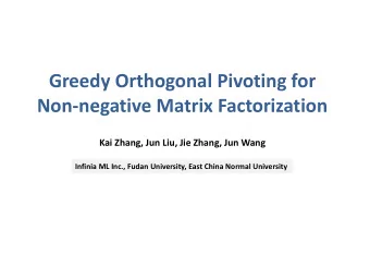
Non-Negative and Geodesic approaches to Independent Component Analysis Mark Plumbley Queen Mary, University of London, Email: mark.plumbley@elec.qmul.ac.uk. ICA Workshop, 20 December 2002.

Overview • Introduction • Nonnegative ICA using nonlinear PCA • Successive rotations • Geodesic line search • Results • Conclusions 1

Introduction • Observations of mixed data - generative model X = AS (1) R n × p and mixing matrix A ∈ I R m × n . with sources S ∈ I • Task - to discover the source samples S and mixing matrix A given only the observations X . • An Underdetermined problem: if ( A ∗ , S ∗ ) is a solution, so is ( A ∗ M , M − 1 S ∗ ) (for invertible M ) • So - need constraints. 2

Constraints 1. Independence of sources: s jk sampled from independent ran- dom variables S j . 2. Non-negativity of sources: s jk ≥ 0 for all 1 ≤ j ≤ n , 1 ≤ k ≤ p . Independence alone → classical noiseless ICA. Non-negativity alone (of S and A ) → non-negative matrix factorization [Lee & Seung, 1999] Both constraints → non-negative independent component analysis . 3

Non-negative ICA using Nonlinear PCA ICA often simplified by pre-whitening - transform x = Qz (2) x ) T ) = I . to get identity covariance C x = E (( x − ¯ x )( x − ¯ Problem now to find orthonormal weight matrix W , satisfying W T W = WW T = I n , such that the outputs y = Wx = WQAs are independent. Typical ICA algorithms search for extremum of contrast function (e.g. kurtosis). 4

Whitening of Non-Negative Data 5 5 4 4 3 3 2 2 x 2 z 2 1 1 0 0 −1 −1 −2 −2 −2 0 2 4 −2 0 2 4 x 1 z 1 (a) (b) Original data (a) is whitened (b) to remove 2nd order correla- tions. Suggests we just try to fit the data into +ve quadrant. 5

Cost/Contrast Function for Non-negative ICA? Let U = WQA , i.e. y = Us For non-negative sources s , which are well-grounded (i.e. Pr( s < δ ) > 0 for any δ > 0), then U is a permutation matrix (i.e. sources are separated) iff all components of y are non-negative w.p.1. So - use a cost function, e.g. mean squared reconstruction error J = 1 x = W T y + 2 E ( � x − ˆ x � ) ˆ where y + is rectified version of y = Wx . 6

Nonlinear PCA algorithms Natural to consider nonlinear PCA algorithm: ∆ W = η g ( y )[ x − Wg ( y )] T in special case of g ( y ) = y + , i.e. ∆ W = η y + [ x − ˆ x = W T y + x ] T ˆ (“non-negative PCA”). Convergence? g ( y ) = y + neither odd nor twice differentiable, so standard proof not applicable. However, behaves like a ‘switching subspace network’, so can modify PCA subspace convergence proofs (to be confirmed!) 7

Orthonormality through Axis Rotation Nonlinear PCA updates W in Euclidean matrix space, tending towards orthonormality WW T = I . However, can instead construct W from 2D rotations [Comon, 1994], � � � � � � y i 1 cos φ sin φ x i 1 = y i 2 -sin φ cos φ x i 2 Rotations (and product) always remain orthonormal. Construct update multiplicatively as W ( t ) = R ( t ) R ( t − 1) · · · R (1) W (0) where R ( t ) is a 2D Givens rotation. 8

2D Axis rotations x 2 x y 1 l y 2 � x 1  0 if y 1 ≥ 0, y 2 ≥ 0    y 2 if y 1 ≥ 0, y 2 < 0   2 2 J = y 2 if y 1 < 0, y 2 ≥ 0 1   y 2 1 + y 2 2 = l 2  otherwise (i.e. y 1 ≥ 0, y 2 < 0)   9

Derivative and Algorithm  0 if y 1 ≥ 0, y 2 ≥ 0   if y 1 ≥ 0, y 2 < 0  y 2 y 1  = dJ/dθ − y 1 y 2 if y 1 < 0, y 2 ≥ 0    0 otherwise ( y 1 ≥ 0, y 2 < 0)  = y + × y − y + 2 − y + 1 y − 2 y − = 1 Gradient descent algorithm: ∆ φ = − η φ · dJ/dφ = + η φ · dJ/dθ η φ ( y + 1 y + 1 y − 2 − y − = 2 ) Relate this to concept of torque in a mechanical system. 10

Line Search over Rotation Angle Instead of simple gradient descent, can use line search. E.g. Matlab fzero for zero of dJ/dφ . If sources are non-negative as required, we know min( J ) = 0 so make local quadratic approximation and jump to φ ( t + 1) = φ ( t ) − 2 J ( t ) / ( dJ ( t ) /dφ ) OK since solution locally quadratic & curvature increases away from solution, as more data points ‘escape’ from the +ve quad- rant. 11

More Than 2 Dimensions: Algorithm 1. Set X (0) = X , W (0) = I , t = 0. 2. Calculate Y = X ( t ) = W ( t ) X (0) k y + ik y + ik y − jk − y − 3. Calculate torques g ij = � jk 4. Exit if | g ij | < tolerance 5. For i ∗ , j ∗ maximizing | g ij | construct X ∗ from selecting rows i ∗ and j ∗ from X ( t ). 6. Do line search to find φ ∗ ( t + 1) which minimizes J . 7. Form the rotation matrix R ( t +1) = [ r ( t +1) ij ] from φ ∗ ( t +1). 8. Form the updated weight matrix W ( t + 1) = R ( t + 1) W ( t ) and modified input data X ( t +1) = R ( t +1) X ( t ) = W ( t +1) X (0). 9. Increment the step count t , and repeat from 2. 12

Geodesic search Successive rotations - equivalent to line search along axis direc- tions. Search in more general directions? Geodesic - shortest path between 2 points on a manifold. For orthonormal matrices, have [Edelmam, Arias & Smith, 1998] W ( τ ) = e τ B W (0) where B T = − B and τ scalar. [Fiori 2001, Nishimori 1999] NB: In 2D we get � � � � 0 b cos( τb ) sin( τb ) e τ B = B = − b 0 − sin( τb ) cos( τb ) 13

Steepest Descent Geodesic Parameterize B = C − C T with c ij = 0 for i ≥ j . C has n ( n − 1) / 2 free parameters. For steepest descent in C space, maximize (distance moved by of τ C due to ∆ τ ) / ∆ τ = dJ/dτ (change in J due to ∆ τ ) / ∆ τ − lim � C � F ∆ τ → 0 We find dJ/dτ = trace(( Y − Y T − YY T − ) C T ) = < ( Y − Y T − YY T − ) , C > so for steepest descent choose C ∝ UT( Y − Y T − YY T − ) = UT( Y − Y T + − Y + Y T − ) 14

Gradient descent Simply update W according to W ( t + 1) = e − η ( Y − Y T + − Y + Y T − ) W ( t ) with small update η . This is the geodesic flow method [Fiori 2001, Nishimori 1999]. BUT - no need to restrict to small updates. Can do e.g. line search along the steepest-descent geodesic. 15

Line Search along Geodesic: Algorithm 1. X (0) = X and W (0) = I at step t = 0. 2. Calculate Y = X ( t ) = W ( t ) X (0). 3. Calculate gradient G ( t ) = UT( Y − Y T + − Y + Y T − ) and B -space movement direction H ( t ) = − ( G ( t ) − G ( t ) T ) = Y + Y T − − Y − Y T + . 4. Stop if � G ( t ) � < tolerance. Perform a line search for τ ∗ which minimizes J ( τ ) using 5. Y ( τ ) = R ( τ ) X ( t ) and R ( τ ) = e − τ H . 6. Update W ( t + 1) = R ( τ ∗ ) W ( t ) and X ( t + 1) = R ( τ ∗ ) X ( t ) = W ( t + 1) X (0). 7. Increment t , repeat from 2. Until exit at 4. For simple tasks can guess single quadratic jump to J = 0 ∆ C = 2 J G / � G � 2 . 16

Results - Image separation problem Source images and histograms [Cichocki, Kasprzak & Amari 1996]. 17

(a) Initial state Nonlinear PCA 0 10 (b) After 50 epochs Error −5 10 −10 10 0 50 100 150 200 Epoch, t (c) After 200 epochs 18

(a) Initial state Successive rotations (b) 5 epochs: rotated axes 1-3 0 10 Error (c) 15 epochs: rotated axes 2-3 −10 10 0 5 10 15 20 25 Epoch 19 (c) 22 epochs: rotated axes 1-3

Geodesic step 0 10 −5 10 Error −10 10 −15 10 0 5 10 15 Epoch (Visually similar images) 20

Music example: Liszt Etude No 5 (extract) 250 200 Frequency bin 150 100 50 50 100 150 200 250 300 350 400 450 Frame 2 Output 4 6 8 10 50 100 150 200 250 300 350 400 450 Frame 21

Conclusions • Considered problem of non-negative ICA • Separation of whitened sources when zero reconstruction er- ror. • Nonlinear PCA with g ( y ) = y + . • Successive rotations keeps orthogonality • Geodesic line search 22