Machine Learning (CSE 446): (continuation of overfitting &) - PowerPoint PPT Presentation
Machine Learning (CSE 446): (continuation of overfitting &) Limits of Learning Sham M Kakade 2018 c University of Washington cse446-staff@cs.washington.edu 1 / 17 Announcement Qz section tomo: (basic) probability and linear
Machine Learning (CSE 446): (continuation of overfitting &) Limits of Learning Sham M Kakade � 2018 c University of Washington cse446-staff@cs.washington.edu 1 / 17
Announcement ◮ Qz section tomo: (basic) probability and linear algebra review ◮ Today: ◮ review ◮ some limits of learning 1 / 17
Review 1 / 17
The “i.i.d.” Supervised Learning Setup ◮ Let ℓ be a loss function ; ℓ ( y, ˆ y ) is our loss by predicting ˆ y when y is the correct output. ◮ Let D ( x, y ) define the (unknown) underlying probability of input/output pair ( x, y ) , in “nature.” We never “know” this distribution. ◮ The training data D = � ( x 1 , y 1 ) , ( x 2 , y 2 ) , . . . , ( x N , y N ) � are assumed to be identical, independently, distributed (i.i.d.) samples from D . ◮ We care about our expected error (i.e. the expected loss, the “true” loss, ...) with regards to the underlying distribution D . ◮ Goal: find a hypothesis which as has “low” expected error, using the training set. 2 / 17
Training error ◮ The training error of hypothesis f is f ’s average error on the training data : N ǫ ( f ) = 1 � ˆ ℓ ( y n , f ( x n )) N n =1 ◮ In contrast, classifier f ’s true expected loss: � ǫ ( f ) = D ( x, y ) · ℓ ( y, f ( x )) = E ( x,y ) ∼D [ ℓ ( y, f ( x ))] ( x,y ) ◮ Idea: Use the training error ˆ ǫ ( f ) as an empirical approximation to ǫ ( f ) . And hope that this approximation is good! ◮ For any fixed f , the training error is an unbiased estimate of the true error. 3 / 17
Overfitting: this is the fundamental problem of ML ◮ Let ˆ f be the output of training algorithm. ◮ The training error of ˆ f is (almost) never an unbiased estimate of the true error. ◮ It is usually a gross underestimate . ◮ The generalization error of our algorithm is its true error - training error : ǫ ( ˆ ǫ ( ˆ f ) − ˆ f ) ◮ Overfitting, more formally: large generalization error means we have overfit . ◮ We would like both : ǫ ( ˆ ◮ our training error, ˆ f ) , to be small ◮ our generalization error to be small ◮ If both occur, then we have low expected error :) ◮ It is usually easy to get one of these two to be small. 4 / 17
Danger: Overfitting overfitting error rate unseen data (lower is better) training data depth of the decision tree 5 / 17
Today’s Lecture 5 / 17
Test sets and Dev. Sets ◮ use test set , i.i.d. data sampled D , to estimate the expected error . ◮ Don’t touch your test data to learn! not for hyperparam tuning, not for modifying your hypothesis! ◮ Keep your test set to always give you accurate (and unbiased) estimates of how good your hypothesis is. ◮ Hyperparameters are params of our algorithm/pseudo-code ◮ sometimes hyperparameters monotonically make our training error lower e.g. decision tree maximal width and maximal depth. ◮ How do we set hyperparams? For some hyperparams: ◮ make a dev set , i.i.d. from D (hold aside some of your training set) ◮ learn with training set (by trying different hyperparams); then check on your dev set. 6 / 17
Example: Avoiding Overfitting by “Early Stopping” in Decision Trees ◮ Set a maximum tree depth d max . (also need to set a maximum width w ) ◮ Only consider splits that decrease error by at least some ∆ . ◮ Only consider splitting a node with more than N min examples. In each case, we have a hyperparameter ( d max , w, ∆ , N min ), which you should tune on development data . 7 / 17
One Limit of Learning: The “No Free Lunch Theorem” ◮ We want a learning algorithm which learns very quickly! ◮ “No Free Lunch Theorem”: (Informally) any learning algorithm that learns with very training set size on one class of problems, must do much worse on another class of problems. ◮ inductive bias: But, we do want to bias our algorithms in certain ways. Let’s see... 8 / 17
An Exercise Following ? , chapter 2. Class A Class B 9 / 17
An Exercise Following ? , chapter 2. Test 10 / 17
Inductive Bias ◮ Just as you had a tendency to focus on a certain type of function f , machine learning algorithms correspond to classes of functions ( F ) and preferences within the class. ◮ You want your algorithm to be “biased” towards the correct classifier. BUT this means it must do worse on other problems. ◮ Example Bias: shallow decision trees: “use a small number of features” favors one type of bias. 11 / 17
Another Limit of Learning: The Bayes Optimal Hypothesis ◮ The best you could hope to do: f ( BO ) ( x ) = argmin ǫ ( f ) f ( x ) You cannot obtain lower loss than ǫ ( f BO ) . ◮ Example: Let’s consider classification: Theorem: For classification (binary or multi-class), the Bayes optimal classifier is: f ( BO ) ( x ) = argmax D ( x, y ) , y and it achieves minimal zero/one error ( ℓ ( y, ˆ y ) = � y � = ˆ y � ) of any classifier. 12 / 17
Proof ◮ Consider (deterministic) f ′ that claims to be better than f ( BO ) and x such that f ( BO ) ( x ) � = f ′ ( x ) . ◮ Probability that f ′ makes an error on this input: �� � − D ( x, f ′ ( x )) . y D ( x, y ) �� � ◮ Probability f ( BO ) makes an error on this input: − D ( x, f ( BO ) ( x )) . y D ( x, y ) ◮ By definition, D ( x, f ( BO ) ( x )) = max D ( x, y ) ≥ D ( x, f ′ ( x )) y �� � �� � − D ( x, f ( BO ) ( x )) ≤ − D ( x, f ′ ( x )) ⇒ D ( x, y ) D ( x, y ) y y ◮ This must hold for all x . Hence f ′ is no better than f ( BO ) . 13 / 17
The Bayes Optimal Hypothesis for the Square Loss ◮ For the quadratic loss and real valued y : ǫ ( f ) = E ( x,y ) ∼D ( y − f ( x )) 2 ◮ Theorem: The Bayes optimal hypothesis for the square loss is: f ( BO ) ( x ) = E [ y | x ] (where the conditional expectation is with respect to D ). 14 / 17
Unavoidable Error ◮ Noise in the features (we don’t want to “fit” the noise!) ◮ Insufficient information in the available features (e.g., incomplete data) ◮ No single correct label (e.g., inconsistencies in the data-generating process) These have nothing to do with your choice of learning algorithm. 15 / 17
General Recipe The cardinal rule of machine learning: Don’t touch your test data. If you follow that rule, this recipe will give you accurate information: 1. Split data into training, development, and test sets. 2. For different hyperparameter settings: 2.1 Train on the training data using those hyperparameter values. 2.2 Evaluate loss on development data. 3. Choose the hyperparameter setting whose model achieved the lowest development data loss. Optionally, retrain on the training and development data together. 4. Evaluate that model on test data. 16 / 17
Design Process for ML Applications example 1 real world goal increase revenue 2 mechanism show better ads 3 learning problem will a user who queries q click ad a ? 4 data collection interaction with existing system 5 collected data query q , ad a , ± click 6 data representation ( q word, a word) pairs 7 select model family decision trees up to 20 8 select training/dev. data September 9 train and select hyperparameters single decision tree 10 make predictions on test set October 11 evaluate error zero-one loss ( ± click) 12 deploy $? 17 / 17
Recommend
More recommend
Explore More Topics
Stay informed with curated content and fresh updates.
