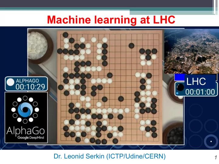
Machine learning at LHC LHC Dr. Leonid Serkin (ICTP/Udine/CERN) 1 - PowerPoint PPT Presentation

Machine learning at LHC LHC Dr. Leonid Serkin (ICTP/Udine/CERN) 1

Introduction 2

Event classification problem (applied to HEP) The question: what ‘decision boundary’ should we use to accept/reject events as belonging to event types H1, H2 or H3? Methods available (up to 2015): Rectangular cut optimization, Projective likelihood estimation, Multidimensional probability density estimation, Multidimensional k-nearest neighbor classifier, Linear discriminant analysis (H-Matrix and Fisher discriminants), Function discriminant analysis, Predictive learning via rule ensembles, Support Vector Machines , Artificial neural network s , Boosted/Bagged decision trees (BDT)… 3

Higgs Boson ML Challenge The Higgs Boson Machine Learning Challenge was organized to promote collaboration between high energy physicists and data scientists. The ATLAS experiment at CERN provided simulated data that has been used by physicists in a search for the Higgs boson. https://www.kaggle.com/c/higgs-boson https://higgsml.lal.in2p3.fr/ 4

Typical neural network circa 2005 An ANN mimics the behaviour of Artificial neuron the biological neuronal networks and consists of an interconnected group of processing elements (referred to as neurons or nodes) arranged in layers. The first layer, known as the input layer, receives the input variables (x1; x2; …xd). Each connection to the neuron is characterised by a weight (w1; w2; … wd) which can be excitatory (positive weight) or inhibitory (negative weight). Moreover, each layer may have a bias (x0 = 1), which can provide a constant shift to the total neuronal input net activation (A), in this case a sigmoid function: 5

Typical neural network circa 2005 The last layer represents the final Artificial neuron response of the ANN, which in the case of d input variables and nH nodes in the hidden layer can be expressed as: The weights and thresholds are the network parameters, whose values are learned during the training phase by looping through the training data several hundreds of times. These parameters are determined by minimising an empirical loss function over all the events N in the training sample and adjusting the weights iteratively in the multidimensional space, such that the deviation E of the actual network output o from the desired (target) output y is minimal 6

Typical neural network circa 2005 ANN architecture: heuristic selection based on complexity adjustment and parameter estimation Theoretical basis: Arnold - Kolmogorov (1957): if f is a multivariate continuous function, then f can be written as a finite composition of continuous functions of a single variable and the binary operation of addition Gorban (1998): it is possible to obtain arbitrarily exact approx. of any continuous function of several variables using operations of summation and multiplication by number, superposition of functions, linear functions and one arbitrary continuous nonlinear function of one variable. 7

Typical neural network circa 2005 ANN architecture: heuristic selection based on complexity adjustment and parameter estimation Theoretical basis: Arnold - Kolmogorov (1957): if f is a multivariate continuous function, then f can be written as a finite composition of continuous functions of a single variable and the binary operation of addition Gorban (1998): it is possible to obtain arbitrarily exact approx. of any continuous function of several variables using operations of summation and multiplication by number, superposition of functions, linear functions and one arbitrary continuous nonlinear function of one variable. An example of a two and three-layer networks with Neural Network is an universal two input nodes. Given an adequate number of approximator for any continuous hidden units, arbitrary nonlinear decision boundaries function 8 between regions R1 and R2 can be achieved

Deep neural network circa 2020 DNN architecture: Structure of the networks, and the node connectivity can be adapted for problem at hand Convolutions: shared weights of neurons, but each neuron only takes subset of inputs Difficult to train, only recently possible with large datasets, fast computing (GPU) and new training procedures / network structures 9 http://www.asimovinstitute.org/neural-network-zoo/

Decision boundaries with TensorFlow https://playground.tensorflow.org 10

Machine learning usage at the LHC • In analysis: – Classifying signal from background, especially in complex final states – Reconstructing heavy particles and improving the energy / mass resolution • In reconstruction: – Improving detector level inputs to reconstruction – Particle identification tasks – Energy / direction calibration • In the trigger: – Quickly identifying complex final states • In computing: – Estimating dataset popularity, and determining needed number and best location of dataset replicas 11

ML@LHC: object reconstruction and calibration 12

ML@LHC: object identification 13

ML@LHC: b-jet identification 14

ML@LHC: candidate particle reconstruction 15

ML@LHC: jet classification 16

Data formats https://arxiv.org/pdf/1807.02876.pdf 17

References https://arxiv.org/pdf/1807.02876.pdf http://www-group.slac.stanford.edu/sluo/Lectures/Stat2006_Lectures.html https://indico.cern.ch/event/77830/ http://www.pp.rhul.ac.uk/~cowan/stat/cowan_weizmann10.pdf https://web.stanford.edu/~hastie/ElemStatLearn/ https://cds.cern.ch/record/2651122 http://cds.cern.ch/record/2634678 http://cds.cern.ch/record/2267879/ 18