M ethode de Monte-Carlo et marche sur les sph` eres pour l - PowerPoint PPT Presentation

Introduction Probabilistic interpretation of L MC algorithms for (LPB) MC algorithm for the nonlinear PB equation M´ ethode de Monte-Carlo et marche sur les sph` eres pour l’´ equation de Poisson-Boltzmann lin´ eaire et non-lin´ eaire de la dynamique mol´ eculaire Nicolas Champagnat, joint work with M. Bossy, D. Talay, L. Violeau, M. Yvinec (Inria Sophia), H. Leman (CMAP, X), S. Maire (Univ. Toulon) S´ eminaire de probabilit´ es, LJK, Grenoble, 20 novembre 2014

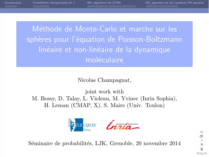
Introduction Probabilistic interpretation of L MC algorithms for (LPB) MC algorithm for the nonlinear PB equation Introduction Poisson-Boltzmann PDE of molecular dynamics The Poisson-Boltzmann (PB) PDE of molecular dynamics is solved by the electrostatic potential around a biomolecular assembly, which is used to compute global characteristics of the system like • the solvatation free energy • the electrostatic forces exerted by the solvent on the molecule. It takes the form of the Poisson equation � div( " ( x ) r u ( x )) +  2 ( x ) sinh u ( x ) = f ( x ) , x 2 R 3 , where • " ( x ) is the permittivity of the medium •  2 ( x ) is called the “ion accessibility parameter”. This is an “implicit solvent” equation, which means that the solvent is considered as a continuum.

Introduction Probabilistic interpretation of L MC algorithms for (LPB) MC algorithm for the nonlinear PB equation Introduction The geometry of the problem The atomic structure of the molecule is modelled in details: • N atoms at positions x 1 , . . . , x N in Ω i with radii r 1 , . . . , r N and charge q i • Ω i = [ N i =1 B ( x i , r i )

Introduction Probabilistic interpretation of L MC algorithms for (LPB) MC algorithm for the nonlinear PB equation Introduction Linear and non-linear PB equations � div( " ( x ) r u ( x )) +  2 ( x ) sinh u ( x ) = f ( x ) , x 2 R 3 , (PB) When the source term is not too big (i.e. when the biomolecule is not very charged), the electrostatic potential can be approximated by the solution of the linearized Poisson-Boltzmann equation � div( " ( x ) r u ( x )) +  2 ( x ) u ( x ) = f ( x ) , x 2 R 3 , (LPB)

Introduction Probabilistic interpretation of L MC algorithms for (LPB) MC algorithm for the nonlinear PB equation Introduction Di ffi culties • The source term is singular N X f := q i � x i . i =1 This di ffi culty can be removed by considering the solution of " i ∆ u = f N 1 q j X u 0 ( x ) = 8 x 2 Ω int . 4 ⇡" int | x � x l | l =1 Then v := u � � u 0 solves PB equation with a smooth source term, if � has compact support in Ω i and ⌘ 1 in the neighborhood of { x 1 , . . . , x N } . •  is discontinuous • The operator has divergence form with discontinuous coe ffi cient " . • Nonlinearity.

Introduction Probabilistic interpretation of L MC algorithms for (LPB) MC algorithm for the nonlinear PB equation Introduction Arguments in favour of a probabilistic resolution method • Dimension 3 • The free energy of the solution of this PDE has the form N 1 X q i ( u � u 0 )( x i ) 2 i =1 • Walk on spheres techniques allow us to deal with the geometry of the molecule e ffi ciently

Introduction Probabilistic interpretation of L MC algorithms for (LPB) MC algorithm for the nonlinear PB equation Introduction Arguments in favour of a probabilistic resolution method • Dimension 3 • The free energy of the solution of this PDE has the form N 1 X q i ( u � u 0 )( x i ) 2 i =1 • Walk on spheres techniques allow us to deal with the geometry of the molecule e ffi ciently This talk deals with two aspects of the problem: • the probabilistic interpretation of the divergence-form operator L := div( " r ) (in any dimension) • the construction of Monte Carlo approximation algorithms based on walk on sphere, appropriate discretization, branching Brownian motion and adapted to the geometry of the problem

Introduction Probabilistic interpretation of L MC algorithms for (LPB) MC algorithm for the nonlinear PB equation What is known in dim 1? The case of dimension 1 The case of dimension 1 is quite well understood (Portenko 1979, Le Gall 1985, Ouknine 1990, several works of Etor´ e, Lejay, Martinez...). Consider the case ( " � if x < 0 " ( x ) = if x � 0 " + Then • L is the infinitesimal generator of the solution of the SDE 2 " ( X t ) dB t + " + � " � p dL 0 dX t = t ( X ) . 2 " + • There is strong existence and pathwise uniqueness for this SDE.

Introduction Probabilistic interpretation of L MC algorithms for (LPB) MC algorithm for the nonlinear PB equation What is known in dim 1? The case of dimension 1 (2) • Two linear scalings of R + and R � transform X into a skew p ε + �p ε � Brownian motion of parameter � = p ε + + p ε � . • Another piecewise linear transformation transforms X into a standard SDE with discontinuous di ff usion coe ffi cient. • Exact simulation schemes are known for skew the Brownian motion: • this is a standard Brownian motion until it hits 0 • the probability to hit h before − h starting from 0 is ( β + 1) / 2 and the hitting time has the same law as for the Brownian motion.

Introduction Probabilistic interpretation of L MC algorithms for (LPB) MC algorithm for the nonlinear PB equation multidimensional SDE with local time Notation We assume that Γ is a smooth ( C 3 ) manifold in R d . We introduce the notations • ⇡ ( x ) for the orthogonal projection of x on Γ • n ( y ) as the outward normal to Γ for y 2 Γ • ⇢ ( x ) as the signed distance between x and Γ ⇢ ( x ) := ( x � ⇡ ( x )) · n ( ⇡ ( x )) .

Introduction Probabilistic interpretation of L MC algorithms for (LPB) MC algorithm for the nonlinear PB equation multidimensional SDE with local time A martingale problem Smooth functions in the domain of L must satisfy the transmission property " int r int ' ( x ) · n ( x ) = " ext r ext ' ( x ) · n ( x ) . We say that ( P x ) x 2 R d on ( C , B ) solves the martingale problem (MP) for L if, for all x 2 R d , one has P x { w 2 C : w (0) = x } = 1 , and, for all ' satisfying b ( R d \ Γ ) , ' 2 C 0 b ( R d ) \ C 2 " r ' · ( n � ⇡ ) 2 C 0 b ( N ) , one has Z t M ϕ t ( w ) := ' ( w ( t )) � ' ( w (0)) � L ' ( w ( s )) ds is a P x martingale. 0

Introduction Probabilistic interpretation of L MC algorithms for (LPB) MC algorithm for the nonlinear PB equation multidimensional SDE with local time The main result Theorem (Bossy, C., Maire, Talay, 2010) The martingale problem for L is well-posed. In addition, there is weak existence and uniqueness in law for the SDE 2 " ( X t ) dB t + " ext � " int 8 p n ( X t ) dL 0 dX t = t ( Y ) , < 2 " ext (1) Y t = ⇢ ( X t ) , : and the corresponding laws solve the MP for L .

Introduction Probabilistic interpretation of L MC algorithms for (LPB) MC algorithm for the nonlinear PB equation multidimensional SDE with local time Ingredients of the proof • We construct a smooth local straightenings of Γ defined on a neighborhood U of x , s.t. 1 = ⇢ and, if ( X t ) solves (1), then Z t := ( X t ) satisfies 2 " ( X t ) dB t + " e � " i dZ 1 p dL 0 t ( Z 1 ) + (drift)( Z t ) dt , t = 2 " e and there is no local time term in the SDE solved by Z 2 t , . . . , Z d t . • Girsanov’s formula allows one to remove the drift term, so that Z 1 t solves a one-dimensional SDE • The SDEs for Z 2 , . . . , Z d can then be solved as time dependent SDEs for all paths of Z 1 • Only weak existence.

Introduction Probabilistic interpretation of L MC algorithms for (LPB) MC algorithm for the nonlinear PB equation multidimensional SDE with local time Ingredients of the proof (continued) Lemma (Generalized Itˆ o-Meyer formula) If X is a continuous semimartingale and if u is a function satisfying the assumption of the MP for L , then Z t Z t 3 @ 2 u r int u ( X s ) · dX s +1 X ( X s ) d h X i , X j i s u ( X t ) = u ( X 0 )+ 2 @ x i @ x j 0 0 i , j =1 Z t + 1 f ( X s ) dL 0 s ( Y ) , 8 t � 0 a.s. , 2 0 ✓ " int ◆ r int u ( ⇡ ( x )) · n ( ⇡ ( x )) . � 1 where f ( x ) = " ext • The formula would be easily obtained from Itˆ o’s and Itˆ o-Tanaka’s formulas for a functions of the form u ( x ) � f ( x )[ ⇢ ( x )] + approximation argument. • If ( X t ) solves (1), the local time terms cancel.

Introduction Probabilistic interpretation of L MC algorithms for (LPB) MC algorithm for the nonlinear PB equation Feynman-Kac formulas Back to linearized Poisson-Boltzmann equation Proposition (Classical Feynman-Kac) Let v be the solution of � div( " r v ) +  2 v = g, where g is a smooth function. Then, for all x 2 R 3 , Z + 1 Z t ✓ ◆ �  2 ( X s ) ds v ( x ) = E x g ( X t ) exp � dt . 0 0 This representation is not very convenient for simulation since • One needs to precisely discretize X everywhere where g is nonzero. • In general, the computation of g is costly. Since X has (scaled) Brownian paths away from Γ , it is better to have formulas only involving informations on the entrance time and position in small neighborhoods of Γ .