M-Estimation in INARCH Models with a special focus on small means - PowerPoint PPT Presentation

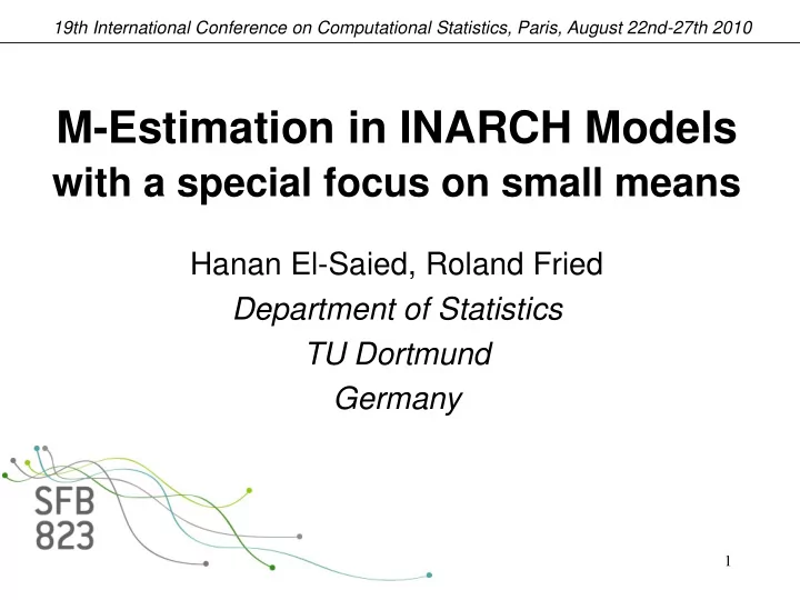
19th International Conference on Computational Statistics, Paris, August 22nd-27th 2010 M-Estimation in INARCH Models with a special focus on small means Hanan El-Saied, Roland Fried Department of Statistics TU Dortmund Germany 1

Contents • Motivation: Outliers in IN(G)ARCH models • M-estimation for i.i.d. Poisson data • M-estimation for INARCH-model • Bias correction • Outlook 2

Motivation: Number of Campylobacterosis Infections 50 40 30 number 20 10 0 0 20 40 60 80 100 120 140 time (4 week periods)      INGARCH-model : Y ~ Poi  Ferland, Latour, Oraichi (2006) t Y , s t t s         Y   t 0 1 t 13 1 t 1 Level shift at time 84, outlier pattern at time 100 Fokianos, F. (2010) 3

● M-estimation of location  for i.i.d. data     n n     y y t t            Minimize         t 1 t 1    e.g. log f gives ML-estimator 4

● M-estimation of location  for i.i.d. data     n n     y y t t            Minimize         t 1 t 1    e.g. log f gives ML-estimator Huber  -function Tukey  -function 3 2 psi-function 2 psi-function 1 1 -3 -2 -1 0 0 -1 -2 -4 -2 0 2 4 x -4 -2 0 2 4 x 2     2 x , | x | k   x             ( x )   ( x ) x 1 I | x | k k   k    k sign ( x ), | x | k   k   5

M-estimation for i.i.d. Poisson data Modified Huber  -function with bias correction     y a      , | y a | k      ( y , ) k , a           k sign ( y a ), | y a | k     with a=a(  ) such that    E Y , 0  Simpson et al. (1987) k , a 1 6

M-estimation for i.i.d. Poisson data Modified Huber  -function with bias correction     y a      , | y a | k      ( y , ) k , a           k sign ( y a ), | y a | k     with a=a(  ) such that    E Y , 0  Simpson et al. (1987) k , a 1 Modified Tukey  -function with bias correction 2   2               y y y 2                 ( y , ) a k a I a k         k , a            Initialization by sample median or by estimating P  (Y=0) 7

Efficiencies: asymptotic and sample size n=50 Asymptotic efficiency of Finite sample efficiency of Huber M-est. for several k Huber & Tukey M-est., n=50 1.00 .8 1.0 asymptotic efficiency relative efficiency .95 .6 .90 .4 .85 .2 .80 .0  0 5 10 15 20 25 0 5 10 15 20 25 huberM (robustbase), k=1.8 k=1 k=2 glmrob, k=1.8 Tukey, k=5 Tukey, k=6 Cadigan & Chen (2001) Tukey, adaptive k 8

Efficiencies: asymptotic and sample size n=50 Asymptotic efficiency of Finite sample efficiency of Huber M-est. for several k Huber & Tukey M-est., n=50 1.00 .8 1.0 asymptotic efficiency relative efficiency .95 .6 .90 .4 .85 .2 .80 .0  0 5 10 15 20 25 0 5 10 15 20 25 huberM (robustbase), k=1.8 k=1 k=2 glmrob, k=1.8 Tukey, k=5 Tukey, k=6 Cadigan & Chen (2001) Tukey, adaptive k 9

Robustness for  =0.5 and  =5 Efficiency relatively to sample mean in case of increasing number of outliers of increasing size, n=50, log-scale 1000 1000 relative efficiency relative efficiency 100 100 10 10 1 1 0.1 0.1 0 5 10 15 20 0 5 10 15 20 number and size of outliers number and size of outliers huberM (robustbase), k=1.8 glmrob, k=1.8 Tukey, k=5 Tukey, k=6 Tukey, adaptive k 10

● Conditional likelihod estimation for INARCH              INARCH-model :  Y ~ Poi , Y Y    t Y , s t t t 0 1 t 1 p t p s Conditioning on first p observations y 1 , …, y p :     1 0         n y     y 1 t 1 t t               t t t p 1       y      0 t p 11

● Conditional likelihod estimation for INARCH              INARCH-model :  Y ~ Poi , Y Y    t Y , s t t t 0 1 t 1 p t p s Conditioning on first p observations y 1 , …, y p :     1 0         n y     y 1 t 1 t t               t t t p 1       y      0 t p   1   M-estimation:     y   t 1               ,  2 marginal     y    t t         mean & variance t       y  t p               12

Efficiencies: INARCH(1),  0 =1,several  1 , n=100 Efficiency for  1 Efficiency for  0 .0 .2 .4 .6 .8 1.01.2 .0 .2 .4 .6 .8 1.01.2 relative efficiency relative efficiency  1 0.0 0.2 0.4 0.6 0.8 0.0 0.2 0.4 0.6 0.8 Huber, k=1.8, Huber, k=2.5 Tukey, k=5, Tukey, k=7 Tukey, adaptive k 13

Robustness: INARCH(1) with  0 =1,  1 =.4 Increasing number k of outliers of size k at end of time series Bias for  0 .1 .0 bias -.1 -.2 -.3 0 5 10 15 20 number and size of outliers Conditional ML Huber, k=1.8, Huber, k=2.5 Tukey, k=5, Tukey, k=7 Tukey, adaptive k 14

Robustness: INARCH(1) with  0 =1,  1 =.4 Increasing number k of outliers of size k at end of time series Bias for  1 Bias for  0 .1 .5 .4 .0 bias bias .3 -.1 .2 -.2 .1 -.3 .0 0 5 10 15 20 0 5 10 15 20 number and size of outliers number and size of outliers Conditional ML Huber, k=1.8, Huber, k=2.5 Tukey, k=5, Tukey, k=7 Tukey, adaptive k 15

● Bias correction for INARCH(p) model M-estimator with bias correction:     1             a 0 y  0    t 1                     n          y 1  t t                         t t   t p 1           y      t p          a   0     p          with a o ,…, a p depending on  0 , …,  p such that expectation of left hand side equals 0. 16

Bias for INARCH(1) in dependence on  1 n=100 .3 .2 Bias  0 .1 Conditional ML .0 Tukey, k=7 -.1  1 Tukey, k=5 .1 .3 .5 .7 .9 Tukey, k=5, corrected .04 -.04 -.02 .00 .02  1 Bias  1 .1 .3 .5 .7 .9 17

Bias for INARCH(1) in dependence on  1 n=200 n=100 .3 .3 .2 .2 Bias Bias  0 .1 .1 Conditional ML .0 .0 Tukey, k=7 -.1 -.1  1 Tukey, k=5 .1 .3 .5 .7 .9 .1 .3 .5 .7 .9 Tukey, k=5, corrected .04 -.04 -.02 .00 .02 .04 Bias correction -.04 -.02 .00 .02  1 Bias Bias effective only in large samples  1 .1 .3 .5 .7 .9 .1 .3 .5 .7 .9 18

Conclusions Tukey M-estimators more robust against many large outliers Needs good robust initialization - from median or P  (Y=0) Adaptive choice of the tuning constant k gives M-estimators with good efficiencies irrespective of the true Poisson parameter M-estimators provide robustness also in INARCH case Bias correction works for long time series Ongoing work: extend to INGARCH, prove asymptotic normality 19

References Cadigan, N.G., Chen, J. (2001). Properties of Robust M-estimators for Poisson and Negative Binomial Data. J. Statist. Comput. Simul. 70, 273-288. Davis, R.A., Dunsmuir, W.T.M., Street, S.B. (2003). Observation driven models for Poisson counts. Biometrika 90, 777-790. Ferland, R.A., Latour, A., Oraichi, D. (2006). Integer-valued GARCH processes. Journal of Time Series Analysis 27, 923-942. Fokianos, K., Fried, R. (2010). Outliers in INGARCH Processes. Journal of Time Series Analysis 31, 210-225 . Fokianos, K., Rahbek, A., Tjøstheim, D. (2009). Poisson Autoregression. J ournal of the American Statistical Association 104, 1430-1439. Simpson, D.G., Carroll, R.J., Ruppert, D. (1987). M-Estimation for Discrete Data: Asymptotic Distribution Theory & Implications. 20 Annals of Statistics 15, 657-669.