LUX PLR Overview Shaun Alsum 1 LUX Goals Discover WIMPs - PowerPoint PPT Presentation
LUX PLR Overview Shaun Alsum 1 LUX Goals Discover WIMPs Necessary requirement: establish inconsistency of LUX results with no-WIMP scenario Set Limits (quantify inconsistency of data with the existance of WIMPs) 2 Profile
LUX PLR Overview Shaun Alsum 1
LUX Goals • Discover WIMPs – Necessary requirement: establish inconsistency of LUX results with no-WIMP scenario • Set Limits (quantify inconsistency of data with the existance of WIMPs) 2
Profile Likelihood Ratio • The PLR is the statistical machinery that accomplishes the above goals • The PLR is nothing more than a prescription for how to choose parameters for, and execute a series of frequentist hypothesis tests . 3
Hypothesis test • Statistical procedure for establishing the consistency or inconsistency of a set of data with a stated hypothesis. • The procedure is as follows: – Precisely state the null hypothesis – Choose a test statistic – Determine the PDF for the null hypothesis as a function of the test statistic – Establish an acceptance/rejection region4 – Compare the test statistic of the measurement to the PDF to determine whether it lies in the acceptance region, or rejection region. 4
Example: verifying a person’s sex by height • Null Hypothesis: person X is a male. • Test statistic: height in inches • PDF Data shown is for males between 20 and 29 years old from a US census survey conducted in 2007 https://www2.census.gov/library/publications/2010/comp endia/statab/130ed/tables/11s0205.pdf 5
Example: verifying a person’s sex by height (continued) • Acceptance/rejection region • Measure the height of person x and compare – (say we measured 72”) 72” lies within our acceptance region, therefore person x is consistent with being male under our statistical test. 6
Hypothesis Tests Improved • Sometimes we have a specific alternative to our null hypothesis we wish to test against. Our test can be improved by stating an alternative hypothesis in addition to our null hypothesis. • There are now two possible errors in our test: – Type 1: the null hypothesis is true and we reject it – Type 2: the alternative hypothesis is true and we reject it • The Significance of a test (typically denoted α ) is the fraction of the time the null hypothesis would be rejected, even if it were true. • The Power of a test is 1 – β , where β is the fraction of the time that the null hypothesis is accepted, even if the alternative hypothesis is true. • The best tests will make both α and β as small as possible. 7
Example: Sex by height revisited • Null Hypothesis (H0): person X is a male. • Alternative Hypothesis (H1): person X is a female. • Test statistic: height in inches • PDF Same deal as before with the data 8
Example: Sex by height revisited (continued) • Acceptance/Rejection Region – Probability of Type 1 error (given H0 true): α – Probability of Type 2 error (given H1 true): β α β • Compare: Say we measure 69” Conclusion: Person X is consistent with being male with significance α . Caution: this does not mean person X has a 1- α probability of being male. 9
Hypothesis Tests: Improved More • Often we can measure more than one observable and would like to use both. In this case, we can choose our test statistic to be a function of multiple observables. • An excellent way (though not the only way) to accomplish this is to use the likelihood of your model given your data as your test statistic. – Note: until this point, our PDF has served only inform our choice of acceptance region (and allow us to report our significance α ). Now we are using it in our calculations; how else are we going to compare quantities of different units? 10
Example: Sex by Height and Weight • Null Hypothesis (H0): person X is a male. • Test Statistic: ℒ 𝑛𝑏𝑚𝑓; (ℎ, 𝑥) = 𝑄 ℎ𝑓𝑗ℎ𝑢 𝑦 ∗ 𝑄 𝑥𝑓𝑗ℎ𝑢 (𝑥) – here I assume height and weight are uncorrelated, clearly a bad assumption, but I didn’t want to deal with it (and didn’t have data in hand). Should have a 2D PDF instead of a product of 2 1-D PDFs • PDF + = 11
Example: Sex by Height and Weight (continued) • Acceptance/Rejection region – accept region of higher likelihood • Compare: say we measure 75” and 250 lbs – Calculate the likelihood of the male model based on this data: 0.00147 Conclusion: person X is inconsistent with being male with significance α 12
Hypothesis Tests: The Final Improvement (Neyman Pearson Lemma) • When using an alternative hypothesis, we want to minimize both α and β . • Neyman Pearson Lemma: For a hypothesis test between two simple hypothesis (hypothesis whose PDFs can be precisely and completely specified), given a choice for either α or β , the choice of test statistic which minimizes the other is the ratio of the null hypothesis’ likelihood to the alternative hypothesis’ likelihood. And the choice of acceptance region is including regions of decreasing likelihood ratio until the remaining fractional area is α . ℒ(𝐼0;𝑦) 𝜇 = ℒ(𝐼1;𝑦) sometimes the test statistic 𝑟 = −2 ln 𝜇 is used 13
Example: Sex by Height and Weight Revisited • Null Hypothesis (H0): person X is a male. • Alternative Hypothesis (H1): person X is a female. ℒ(𝐼0;(ℎ,𝑥)) • Test Statistic: 𝜇 = ℒ(𝐼1;(ℎ,𝑥)) • PDF: Percent of + people Height [inches] Overflow 14
Example: Sex by Height and Weight Revisited (continued) • Acceptance/Rejection region: binning too large to represent accurately, but essentially rejection region is a fraction of the left bin if we choose α = 0.05 • Compare: say that again we measure 75 ” and 250 lbs Conclusion: Person X is consistent with being male Data comparison 15
Hypothesis Tests: Extension to Non- simple Hypothesis • What if we cannot specify our PDFs precisely? (as is actually most often the case in reality) • the most likely model for the null and alternative hypotheses given the data in the likelihood ratio instead of a-priori determined PDFs. – Parameterize the PDFs in terms of nuisance parameters. – Choose the values of these parameters (independently for the null and alternative hypotheses) such that the likelihood for the null hypothesis in the numerator is maximized, and again so that the likelihood for the alternative hypothesis in the denominator is maximized. – If one has an idea of what these nuisance parameters might be, a term can be added to the likelihood function, profiling the parameter, typically decreasing the likelihood the further the parameter is from its expected value. 16
Example: Counting Experiment • Suppose one wants to determine whether the activation of a beam causes a signal in a detector. • The detector takes measurements for an amount of time T without the beam turned on and measures m events • The detector then takes measurements for an amount of time T with the beam turned on and measures n events. • Null hypothesis: the beam creates no signal • Alternative hypothesis: the beam adds, on average, p events per time T • Test statistic: likelihood ratio – Likelihood function no profiling: 𝑄𝑝𝑗𝑡 𝑜; 𝑐 + 𝑡 ∗ 𝑞 ∗ 𝑄𝑝𝑗𝑡(𝑛; 𝑐) where s = 0 for the null hypothesis and s = 1 for the alternative hypothesis – Likelihood function with profiling: 𝑄𝑝𝑗𝑡 𝑜; 𝑐 + 𝑡 ∗ 𝑞 ∗ 𝑄𝑝𝑗𝑡(𝑛; 𝑐) *Gaus(b; b exp , b std ) Nuisance parameters: b 17
PLR: Generating the PDF • We already stated that in our use case, we cannot determine the PDFs for the null or alternative hypotheses completely, so how do we proceed? • Toy Monte Carlos: Generate data sets from our models using values of nuisance parameters drawn from our profiling. • The collection of test statistics calculated from these toy mcs forms our PDF. 18
Example: Counting Experiment (Continued) • PDF: Red: signal + background Blue: background only # toy mcs Black: data n = 15, m=20 (but bkg only run went for 2T) p = 5 s = 1.1 q (test statistic, -2ln( λ )) 19
Using the PLR to Discover a WIMP • Null hypothesis (H 0 ): There are no WIMPs (parameter of interest = 0). • Alternative hypothesis (H 1 ): There are WIMPs (parameter of interest ≠ 0). ) ℒ(𝜈=0; 𝜄 • Test Statistic: 𝜇 = ) , 𝑟 = −2 ln 𝜇 ℒ(𝜈≠0;𝜄 – Numerator: fix POI (represented by μ ), let all other nuisance parameters (represented by θ ) float and maximize. – Denominator: POI float in addition to all nuisance parameters • The single vs double hat only serves to represent that the values settled on for the nuisance parameters need not be the same in the two likelihood expressions. • Our significance for discovery is chosen to be 5 σ , or α = 3x10 -7 . 20
Recommend
More recommend
Explore More Topics
Stay informed with curated content and fresh updates.


