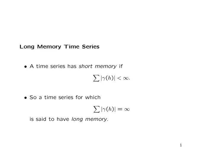
Long Memory Time Series A time series has short memory if | ( h ) - PowerPoint PPT Presentation

Long Memory Time Series • A time series has short memory if � | γ ( h ) | < ∞ . • So a time series for which � | γ ( h ) | = ∞ is said to have long memory . 1

Why do we care? • Write the mean of x 1 , x 2 , . . . , x n as x n = x 1 + x 2 + · · · + x n ¯ . n • Then n − 1 � � x n ) = 1 1 − | h | � var(¯ γ ( h ) n n h = − ( n − 1) ∞ � � = 1 1 − | h | � γ ( h ) n n + h = −∞ where ( a ) + = max( a, 0) is a if a ≥ 0 and 0 if a < 0. 2

• If � | γ ( h ) | < ∞ , then ∞ ∞ � � 1 − | h | � � γ ( h ) → γ ( h ) n + h = −∞ h = −∞ as n → ∞ . • So ∞ � n var(¯ x n ) → γ ( h ) , h = −∞ or   ∞ x n ) = 1 � 1 �  + o � var(¯ γ ( h ) .  n n h = −∞ 3

• That is, for a short memory time series, var(¯ x n ) goes to zero as the sample size increases at the usual rate, σ 2 /n , but with a different multiplier. • Note that ∞ � γ ( h ) = f (0) , h = −∞ the spectral density f ( ω ) evaluated at ω = 0. • So we can also write x n ) = f (0) � 1 � var(¯ + o : n n σ 2 is replaced by f (0). 4

• But if � | γ ( h ) | = ∞ , this doesn’t work. • In practice, many series show var(¯ x n ) decaying more slowly. Plot log[var(¯ x n )] against log( n ), and look for a slope of − 1. vartime = function(x, nmax = round(length(x) / 10)) { v = rep(NA, nmax); for (n in 1:nmax) { y = filter(x, rep(1/n, n), sides = 1); v[n] = var(y, na.rm = TRUE); } plot(log(1:nmax), log(v)); lmv = lm(log(v) ~ log(1:nmax)); abline(lmv); title(paste(deparse(substitute(x)), "; nmax = ", nmax)); print(summary(lmv)); } vartime(log(varve)) vartime(globtemp) vartime(residuals(lm(globtemp ~ time(globtemp)))) 5

Fractional Integration • How can we model such series? • Fractionally integrated white noise: (1 − B ) d x t = w t , 0 < d < 0 . 5 . • ACF is ρ ( h ) = Γ( h + d )Γ(1 − d ) Γ( h − d + 1)Γ( d ) ∼ h 2 d − 1 • So for 0 < d < 0 . 5, ∞ � | ρ ( h ) | = ∞ . h = −∞ 6

Notes: x n ) decays like n (2 d − 1) , so • var(¯ d = 1 + slope of variance-time graph 2 gives a rough empirical estimate of d . • The spectral density is σ 2 w f ( ω ) = � d , � 4 sin( πω ) 2 so for d > 0, f ( ω ) → ∞ as ω → 0. 7

• Also f ( ω ) ∼ | ω | − 2 d as ω → 0, so a graph of log[ f ( ω )] against log( | ω | ) gives another estimate of d . • If d ≥ 0 . 5, f ( ω ) is not integrable, so the series is not station- ary. 8

ARFIMA Model • In some long-memory series, autocorrelations at small lags do not match those of fractionally integrated noise. • We can add ARMA components to allow for such differences; the ARIMA( p, d, q ) model with fractional d , or ARFIMA. • Use the R function fracdiff() : library(fracdiff) summary(fracdiff(log(varve))) summary(fracdiff(log(varve), nar = 1, nma = 1)) summary(fracdiff(residuals(lm(globtemp ~ time(globtemp))))) 9

Trend Estimation with ARFIMA errors • The R function fracdiff() does not allow explanatory vari- ables, but we can use it to calculate a profile likelihood func- tion. • E.g. global temperature versus cumulative CO 2 emissions: source("http://www.stat.ncsu.edu/people/bloomfield/courses/st730/co2w.R"); plot(cbind(globtemp, co2w)); slopes = seq(from = 0, to = 1.5, length = 151); ll2 = rep(NA, length(slopes)); for (i in 1:length(slopes)) ll2[i] = -2 * fracdiff(globtemp - slopes[i] * co2w)$log.likelihood; plot(slopes, ll2, type = "l"); abline(h = min(ll2) + qchisq(.95, 1)); 10

• The point estimate is slopeEst = slopes[which.min(ll2)]; abline(v = slopeEst, col = "red"); # [1] 0.68 and the 95% confidence interval is roughly: slopeCI = range(slopes[ll2 <= min(ll2) + qchisq(.95, 1)]); abline(v = slopeCI, col = "red", lty = 2); # [1] 0.41 1.03 • The CO 2 series was scaled by its change from 1900 to 2000, so we estimate the 20 th century warming as 0 . 68 ◦ C, with a confidence interval of (0 . 41 ◦ C , 1 . 03 ◦ C) (note the asymmetry: 0 . 68( − 0 . 27 , +0 . 35) ◦ C). • Compare with IPCC: 1906–2005 warming is 0 . 74 ◦ C ± 0 . 18 ◦ C. 11