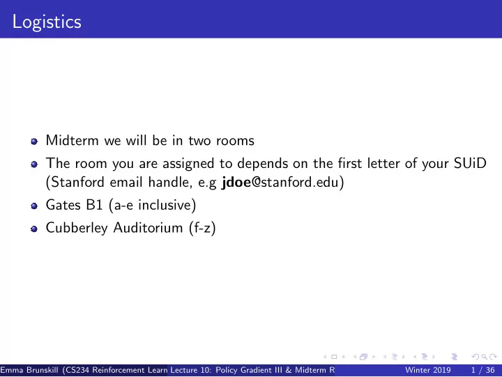
Logistics Midterm we will be in two rooms The room you are assigned - PowerPoint PPT Presentation
Logistics Midterm we will be in two rooms The room you are assigned to depends on the first letter of your SUiD (Stanford email handle, e.g jdoe @stanford.edu) Gates B1 (a-e inclusive) Cubberley Auditorium (f-z) Lecture 10: Policy Gradient III
Logistics Midterm we will be in two rooms The room you are assigned to depends on the first letter of your SUiD (Stanford email handle, e.g jdoe @stanford.edu) Gates B1 (a-e inclusive) Cubberley Auditorium (f-z) Lecture 10: Policy Gradient III & Midterm Review 1 Emma Brunskill (CS234 Reinforcement Learning. ) Winter 2019 1 / 36
Lecture 10: Policy Gradient III & Midterm Review 1 Emma Brunskill CS234 Reinforcement Learning. Winter 2019 Additional reading: Sutton and Barto 2018 Chp. 13 1 With many policy gradient slides from or derived from David Silver and John Schulman and Pieter Abbeel Lecture 10: Policy Gradient III & Midterm Review 1 Emma Brunskill (CS234 Reinforcement Learning. ) Winter 2019 2 / 36
Class Structure Last time: Policy Search This time: Policy Search & Midterm Review Next time: Midterm Lecture 10: Policy Gradient III & Midterm Review 1 Emma Brunskill (CS234 Reinforcement Learning. ) Winter 2019 3 / 36
Recall: Policy-Based RL Policy search: directly parametrize the policy π θ ( s , a ) = P [ a | s ; θ ] Goal is to find a policy π with the highest value function V π Focus on policy gradient methods Lecture 10: Policy Gradient III & Midterm Review 1 Emma Brunskill (CS234 Reinforcement Learning. ) Winter 2019 4 / 36
”Vanilla” Policy Gradient Algorithm Initialize policy parameter θ , baseline b for iteration=1 , 2 , · · · do Collect a set of trajectories by executing the current policy At each timestep t in each trajectory τ i , compute t = � T − 1 Return G i t ′ = t r i t ′ , and Advantage estimate ˆ A i t = G i t − b ( s t ). t || 2 , Re-fit the baseline, by minimizing � � t || b ( s t ) − G i i Update the policy, using a policy gradient estimate ˆ g , Which is a sum of terms ∇ θ log π ( a t | s t , θ ) ˆ A t . (Plug ˆ g into SGD or ADAM) endfor Lecture 10: Policy Gradient III & Midterm Review 1 Emma Brunskill (CS234 Reinforcement Learning. ) Winter 2019 5 / 36
Choosing the Target G i t is an estimation of the value function at s t from a single roll out Unbiased but high variance Reduce variance by introducing bias using bootstrapping and function approximation Just like in we saw for TD vs MC, and value function approximation Estimate of V / Q is done by a critic Actor-critic methods maintain an explicit representation of policy and the value function, and update both A3C (Mnih et al. ICML 2016) is a very popular actor-critic method Lecture 10: Policy Gradient III & Midterm Review 1 Emma Brunskill (CS234 Reinforcement Learning. ) Winter 2019 6 / 36
”Vanilla” Policy Gradient Algorithm Initialize policy parameter θ , baseline b for iteration=1 , 2 , · · · do Collect a set of trajectories by executing the current policy At each timestep t in each trajectory τ i , compute Target ˆ R i t Advantage estimate ˆ A i t = G i t − b ( s t ). t || b ( s t ) − ˆ t || 2 , R i Re-fit the baseline, by minimizing � � i Update the policy, using a policy gradient estimate ˆ g , Which is a sum of terms ∇ θ log π ( a t | s t , θ ) ˆ A t . ( Plug ˆ g into SGD or ADAM ) endfor Lecture 10: Policy Gradient III & Midterm Review 1 Emma Brunskill (CS234 Reinforcement Learning. ) Winter 2019 7 / 36
Policy Gradient Methods with Auto-Step-Size Selection Can we automatically ensure the updated policy π ′ has value greater than or equal to the prior policy π : V π ′ ≥ V π ? Consider this for the policy gradient setting, and hope to address this by modifying step size Lecture 10: Policy Gradient III & Midterm Review 1 Emma Brunskill (CS234 Reinforcement Learning. ) Winter 2019 8 / 36
Objective Function Goal: find policy parameters that maximize value function 1 � ∞ � � γ t R ( s t , a t ); π θ V ( θ ) = E π θ t =0 where s 0 ∼ µ ( s 0 ), a t ∼ π ( a t | s t ) , s t +1 ∼ P ( s t +1 | s t , a t ) Have access to samples from the current policy π θ old (param. by θ old ) Want to predict the value of a different policy (off policy learning!) 1 For today we will primarily consider discounted value functions Lecture 10: Policy Gradient III & Midterm Review 1 Emma Brunskill (CS234 Reinforcement Learning. ) Winter 2019 9 / 36
Objective Function Goal: find policy parameters that maximize value function 1 � ∞ � � γ t R ( s t , a t ); π θ V ( θ ) = E π θ t =0 where s 0 ∼ µ ( s 0 ), a t ∼ π ( a t | s t ) , s t +1 ∼ P ( s t +1 | s t , a t ) Express expected return of another policy in terms of the advantage over the original policy � ∞ � V (˜ � � � γ t A π ( s t , a t ) θ ) = V ( θ ) + E π ˜ = V ( θ ) + µ ˜ π ( s ) π ( a | s ) A π ( s , a ) ˜ θ t =0 s a where µ ˜ π ( s ) is defined as the discounted weighted frequency of state s under policy ˜ π (similar to in Imitation Learning lecture) We know the advantage A π and ˜ π But we can’t compute the above because we don’t know µ ˜ π , the state distribution under the new proposed policy 1 For today we will primarily consider discounted value functions Lecture 10: Policy Gradient III & Midterm Review 1 Emma Brunskill (CS234 Reinforcement Learning. ) Winter 2019 10 / 36
Table of Contents Updating the Parameters Given the Gradient: Local Approximation 1 Updating the Parameters Given the Gradient: Trust Regions 2 Updating the Parameters Given the Gradient: TRPO Algorithm 3 Lecture 10: Policy Gradient III & Midterm Review 1 Emma Brunskill (CS234 Reinforcement Learning. ) Winter 2019 11 / 36
Local approximation Can we remove the dependency on the discounted visitation frequencies under the new policy? Substitute in the discounted visitation frequencies under the current policy to define a new objective function: � � L π (˜ π ) = V ( θ ) + µ π ( s ) π ( a | s ) A π ( s , a ) ˜ s a Note that L π θ 0 ( π θ 0 ) = V ( θ 0 ) Gradient of L is identical to gradient of value function at policy parameterized evaluated at θ 0 : ∇ θ L π θ 0 ( π θ ) | θ = θ 0 = ∇ θ V ( θ ) | θ = θ 0 Lecture 10: Policy Gradient III & Midterm Review 1 Emma Brunskill (CS234 Reinforcement Learning. ) Winter 2019 12 / 36
Conservative Policy Iteration Is there a bound on the performance of a new policy obtained by optimizing the surrogate objective? Consider mixture policies that blend between an old policy and a different policy π new ( a | s ) = (1 − α ) π old ( a | s ) + απ ′ ( a | s ) In this case can guarantee a lower bound on value of the new π new : 2 ǫγ V π new ≥ L π old ( π new ) − (1 − γ ) 2 α 2 � � where ǫ = max s � E a ∼ π ′ ( a | s ) [ A π ( s , a )] � Lecture 10: Policy Gradient III & Midterm Review 1 Emma Brunskill (CS234 Reinforcement Learning. ) Winter 2019 13 / 36
Find the Lower-Bound in General Stochastic Policies Would like to similarly obtain a lower bound on the potential performance for general stochastic policies (not just mixture policies) Recall L π (˜ π ) = V ( θ ) + � s µ π ( s ) � a ˜ π ( a | s ) A π ( s , a ) Theorem Let D max TV ( π 1 , π 2 ) = max s D TV ( π 1 ( ·| s ) , π 2 ( ·| s )) . Then 4 ǫγ V π new ≥ L π old ( π new ) − (1 − γ ) 2 ( D max TV ( π old , π new )) 2 where ǫ = max s , a | A π ( s , a ) | . Lecture 10: Policy Gradient III & Midterm Review 1 Emma Brunskill (CS234 Reinforcement Learning. ) Winter 2019 14 / 36
Find the Lower-Bound in General Stochastic Policies Would like to similarly obtain a lower bound on the potential performance for general stochastic policies (not just mixture policies) π ) = V ( θ ) + � s µ π ( s ) � Recall L π (˜ a ˜ π ( a | s ) A π ( s , a ) Theorem Let D max TV ( π 1 , π 2 ) = max s D TV ( π 1 ( ·| s ) , π 2 ( ·| s )) . Then 4 ǫγ V π new ≥ L π old ( π new ) − (1 − γ ) 2 ( D max TV ( π old , π new )) 2 where ǫ = max s , a | A π ( s , a ) | . Note that D TV ( p , q ) 2 ≤ D KL ( p , q ) for prob. distrib p and q . Then the above theorem immediately implies that 4 ǫγ V π new ≥ L π old ( π new ) − (1 − γ ) 2 D max KL ( π old , π new ) where D max KL ( π 1 , π 2 ) = max s D KL ( π 1 ( ·| s ) , π 2 ( ·| s )) Lecture 10: Policy Gradient III & Midterm Review 1 Emma Brunskill (CS234 Reinforcement Learning. ) Winter 2019 15 / 36
Guaranteed Improvement 1 Goal is to compute a policy that maximizes the objective function defining the lower bound: 1 L π (˜ π ) = V ( θ ) + � s µ π ( s ) � a ˜ π ( a | s ) A π ( s , a ) Lecture 10: Policy Gradient III & Midterm Review 1 Emma Brunskill (CS234 Reinforcement Learning. ) Winter 2019 16 / 36
Guaranteed Improvement 1 Goal is to compute a policy that maximizes the objective function defining the lower bound: 4 ǫγ (1 − γ ) 2 D max M i ( π ) = L π i ( π ) − KL ( π i , π ) 4 ǫγ V π i +1 (1 − γ ) 2 D max ≥ L π i ( π ) − KL ( π i , π ) = M i ( π i +1 ) V π i = M i ( π i ) V π i +1 − V π i ≥ M i ( π i +1 ) − M i ( π i ) So as long as the new policy π i +1 is equal or an improvement compared to the old policy π i with respect to the lower bound, we are guaranteed to to monotonically improve! The above is a type of Minorization-Maximization (MM) algorithm 1 L π (˜ π ) = V ( θ ) + � s µ π ( s ) � a ˜ π ( a | s ) A π ( s , a ) Lecture 10: Policy Gradient III & Midterm Review 1 Emma Brunskill (CS234 Reinforcement Learning. ) Winter 2019 17 / 36
Recommend
More recommend
Explore More Topics
Stay informed with curated content and fresh updates.
