A Composite Randomized Incremental Gradient Method Junyu Zhang - PowerPoint PPT Presentation

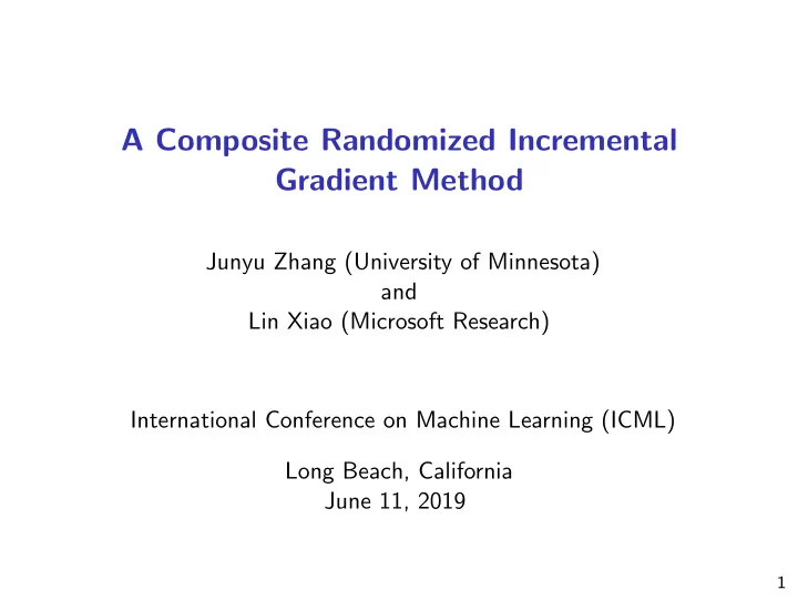
A Composite Randomized Incremental Gradient Method Junyu Zhang (University of Minnesota) and Lin Xiao (Microsoft Research) International Conference on Machine Learning (ICML) Long Beach, California June 11, 2019 1

Composite finite-sum optimization • problem of focus � 1 n � � minimize f g i ( x ) + r ( x ) n x ∈ R d i =1 – f : R p → R smooth and possibly nonconvex – g i : R d → R p smooth vector mapping, i = 1 , . . . , n – r : R d → R ∪ {∞} convex but possibly nonsmooth 2

Composite finite-sum optimization • problem of focus � 1 n � � minimize f g i ( x ) + r ( x ) n x ∈ R d i =1 – f : R p → R smooth and possibly nonconvex – g i : R d → R p smooth vector mapping, i = 1 , . . . , n – r : R d → R ∪ {∞} convex but possibly nonsmooth • extensions for two-level finite-sum problem m n � 1 � 1 � � minimize g i ( x ) + r ( x ) f j m n x ∈ R d j =1 i =1 • applications beyond ERM – reinforcement learning (policy evaluation) – risk-averse optimization, financial mathematics – . . . 2

Examples • policy evaluation with linear function approximation � � � 2 minimize x ∈ R d � E [ A ] x − E [ b ] A , b random, generated by MDP under fixed policy 3

Examples • policy evaluation with linear function approximation � � � 2 minimize x ∈ R d � E [ A ] x − E [ b ] A , b random, generated by MDP under fixed policy • risk-averse optimization n n � n � 2 1 − λ 1 h j ( x ) − 1 � � � maximize h j ( x ) h i ( x ) n n n x ∈ R d j =1 j =1 i =1 � �� � � �� � average reward variance of rewards (risk) – often treated as two-level composite finite-sum optimization 3

Examples • policy evaluation with linear function approximation � � � 2 minimize x ∈ R d � E [ A ] x − E [ b ] A , b random, generated by MDP under fixed policy • risk-averse optimization n n � n � 2 1 − λ 1 h j ( x ) − 1 � � � maximize h j ( x ) h i ( x ) n n n x ∈ R d j =1 j =1 i =1 � �� � � �� � average reward variance of rewards (risk) – often treated as two-level composite finite-sum optimization – simple transformation using Var ( a ) = E [ a 2 ] − ( E [ a ]) 2 n � 1 n � 1 n � 2 � 1 � � � h 2 maximize h j ( x ) − λ j ( x ) − h i ( x ) n n n x ∈ R d j =1 j =1 i =1 actually a one-level composite finite-sum problem 3

Technical challenge and related work • challenge: biased gradient estimator � n – denote F ( x ) := f ( g ( x )) where g ( x ) := 1 i =1 g i ( x ) n F ′ ( x ) = [ g ′ ( x )] T f ′ ( g ( x )) – subsampled estimators y = 1 z = 1 � � g ′ g i ( x ) , i ( x ) , where S ⊂ { 1 , . . . , n } |S| |S| i ∈S i ∈S � � [ z ] T f ′ ( y ) E [ y ] = g ( x ) and E [ z ] = g ′ ( x ), but E � = F ′ ( x ) 4

Technical challenge and related work • challenge: biased gradient estimator � n – denote F ( x ) := f ( g ( x )) where g ( x ) := 1 i =1 g i ( x ) n F ′ ( x ) = [ g ′ ( x )] T f ′ ( g ( x )) – subsampled estimators y = 1 z = 1 � � g ′ g i ( x ) , i ( x ) , where S ⊂ { 1 , . . . , n } |S| |S| i ∈S i ∈S � � [ z ] T f ′ ( y ) E [ y ] = g ( x ) and E [ z ] = g ′ ( x ), but E � = F ′ ( x ) • related work – more general composite stochastic optimization (Wang, Fang & Liu 2017; Wang, Liu & Fang 2017; . . . ) – two-level composite finite-sum: extending SVRG (Lian, Wang & Liu 2017; Huo, Gu, Liu & Huang 2018; Lin, Fan, Wang & Jordan 2018; . . . ) 4

Main results • composite-SAGA: single loop vs double loops of composite-SVRG 5

Main results • composite-SAGA: single loop vs double loops of composite-SVRG � �G ( x t ) � 2 � ≤ ǫ (with G = F ′ if r ≡ 0) • sample complexity for E � n + n 2 / 3 ǫ − 1 � – nonconvex smooth f and g i : O � ( n + κ n 2 / 3 ) log ǫ − 1 � – + gradient dominant or strongly convex: O same as SVRG/SAGA for nonconvex finite-sum problems (Allen-Zhu & Hazan 2016; Reddi et al. 2016; Let et al. 2017) 5

Main results • composite-SAGA: single loop vs double loops of composite-SVRG � �G ( x t ) � 2 � ≤ ǫ (with G = F ′ if r ≡ 0) • sample complexity for E � n + n 2 / 3 ǫ − 1 � – nonconvex smooth f and g i : O � ( n + κ n 2 / 3 ) log ǫ − 1 � – + gradient dominant or strongly convex: O same as SVRG/SAGA for nonconvex finite-sum problems (Allen-Zhu & Hazan 2016; Reddi et al. 2016; Let et al. 2017) • extensions to two-level problem � m + n + ( m + n ) 2 / 3 ǫ − 1 � – nonconvex smooth f and g i : O (same as composite-SVRG (Huo et al. 2018)) – + gradient dominant or optimally strongly convex: � ( m + n + κ ( m + n ) 2 / 3 ) log ǫ − 1 � O (better than composite-SVRG (Lian et al. 2017)) 5

Composite SAGA algorithm (C-SAGA) • input: x 0 ∈ R d , α 0 i for i = 1 , . . . , n , and step size η > 0 � n � n • initialize Y 0 = 1 i =1 g i ( α 0 Z 0 = 1 i =1 g ′ i ( α 0 i ) , i ) n n • for t = 0 , ..., T − 1 – sample with replacement S t ⊂ { 1 , ..., n } with |S t | = s � � y t = Y t + 1 j ∈S t ( g j ( x t ) − g j ( α t j )) s – compute � z t = Z t + 1 j ∈S t ( g ′ j ( x t ) − g ′ j ( α t j )) s � �� � – x t +1 = prox η x t − η z T t f ′ ( y t ) r = x t if j ∈ S t and α t +1 – update α t +1 = α t j otherwise j j � � Y t +1 = Y t + 1 j ∈S t ( g j ( x t ) − g j ( α t j )) n – update � Z t +1 = Z t + 1 j ∈S t ( g ′ j ( x t ) − g ′ j ( α t j )) n • output: randomly choose t ∗ ∈{ 1 , ..., T } and output x t ∗ 6

Convergence analysis � 1 n � � minimize g i ( x ) + r ( x ) f n x ∈ R d i =1 � �� � F ( x ) • assumptions – f is ℓ f -Lipschitz and f ′ is L f -Lipschitz – g i is ℓ g -Lipschitz and g ′ i is L g -Lipschitz, i = 1 , . . . , n – r convex but can be non-smooth implication: F ′ is L F -Lipschitz with L F = ℓ 2 g L f + ℓ f L g 7

Convergence analysis � 1 n � � minimize g i ( x ) + r ( x ) f n x ∈ R d i =1 � �� � F ( x ) • assumptions – f is ℓ f -Lipschitz and f ′ is L f -Lipschitz – g i is ℓ g -Lipschitz and g ′ i is L g -Lipschitz, i = 1 , . . . , n – r convex but can be non-smooth implication: F ′ is L F -Lipschitz with L F = ℓ 2 g L f + ℓ f L g � �G ( x t ) � 2 � • sample complexity for E ≤ ǫ , where G ( x ) = 1 � � �� x − prox η x − η F ′ ( x ) = F ′ ( x ) if r ≡ 0 r η � � � � – if s = 1 and η = O 1 / ( nL F ) , then complexity O n /ǫ � � � � – if s = n 2 / 3 and η = O n + n 2 / 3 /ǫ 1 / L F , then complexity O 7

Linear convergence results • gradient-dominant functions � 1 � n � – assumption: r ≡ 0 and F ( x ) := f i =1 g i ( x ) satisfies n y F ( y ) ≤ ν 2 � F ′ ( x ) � 2 , ∀ x ∈ R d F ( x ) − inf – if s = n 2 / 3 and η = O (1 / L F ), complexity O � ( n + ν n 2 / 3 ) log ǫ − 1 � • optimally strongly convex functions – assumption: Φ( x ) := F ( x ) + r ( x ) satisfies Φ( x ) − Φ( x ⋆ ) ≥ µ 2 � x − x ⋆ � 2 , ∀ x ∈ R d � ( n + µ − 1 n 2 / 3 ) log ǫ − 1 � – if s = n 2 / 3 and η = O (1 / L F ), complexity O � ( m + n + κ ( m + n ) 2 / 3 ) log ǫ − 1 � • extension to two-level case: O 8

Experiments • risk-averse optimization n = 5000, d = 500 n = 5000, d = 500 10 4 10 4 10 2 10 2 (F(x k )+r(x k )) - (F(x*)+r(x*)) 10 0 F(x k ) + r(x k )|| 10 0 10 -2 10 -4 10 -2 || 10 -6 10 -4 C-SAGA C-SAGA 10 -8 ASC-PG ASC-PG VRSC-PG VRSC-PG 10 -6 10 -10 0 0.5 1 1.5 2 2.5 3 0 0.5 1 1.5 2 2.5 3 # of samples 10 5 # of samples 10 5 • policy evaluation for MDP S = 100 S = 100 10 4 10 5 10 2 10 0 10 0 F(w k )- F(w*) F(w k )|| 10 -5 10 -2 || SCGD SCGD 10 -10 ASCGD ASCGD 10 -4 ASC-PG ASC-PG C-SAGA C-SAGA VRSC-PG VRSC-PG 10 -6 10 -15 0 1000 2000 3000 4000 5000 0 1000 2000 3000 4000 5000 # of samples # of samples 9