Local Search Distances Landscape Characteristics Fitness-Distance - PowerPoint PPT Presentation
Outline DM811 1. Local Search, Basic Elements HEURISTICS AND LOCAL SEARCH ALGORITHMS Components and Algorithms FOR COMBINATORIAL OPTIMZATION Beyond Local Optima Computational Complexity 2. Fundamental Search Space Properties Introduction
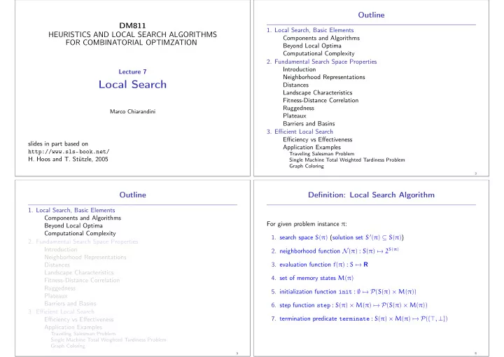
Outline DM811 1. Local Search, Basic Elements HEURISTICS AND LOCAL SEARCH ALGORITHMS Components and Algorithms FOR COMBINATORIAL OPTIMZATION Beyond Local Optima Computational Complexity 2. Fundamental Search Space Properties Introduction Lecture 7 Neighborhood Representations Local Search Distances Landscape Characteristics Fitness-Distance Correlation Ruggedness Marco Chiarandini Plateaux Barriers and Basins 3. Efficient Local Search Efficiency vs Effectiveness slides in part based on Application Examples http://www.sls-book.net/ Traveling Salesman Problem H. Hoos and T. Stützle, 2005 Single Machine Total Weighted Tardiness Problem Graph Coloring 2 Outline Definition: Local Search Algorithm 1. Local Search, Basic Elements Components and Algorithms For given problem instance π : Beyond Local Optima Computational Complexity 1. search space S ( π ) (solution set S ′ ( π ) ⊆ S ( π ) ) 2. Fundamental Search Space Properties Introduction 2. neighborhood function N ( π ) : S ( π ) � → 2 S ( π ) Neighborhood Representations 3. evaluation function f ( π ) : S � → R Distances Landscape Characteristics 4. set of memory states M ( π ) Fitness-Distance Correlation Ruggedness 5. initialization function init : ∅ � → P ( S ( π ) × M ( π )) Plateaux Barriers and Basins 6. step function step : S ( π ) × M ( π ) � → P ( S ( π ) × M ( π )) 3. Efficient Local Search 7. termination predicate terminate : S ( π ) × M ( π ) � → P ( { ⊤ , ⊥ } ) Efficiency vs Effectiveness Application Examples Traveling Salesman Problem Single Machine Total Weighted Tardiness Problem Graph Coloring 3 5
Example: Uninformed random walk for SAT (1) Example: Uninformed random walk for SAT (continued) ◮ search space S : set of all truth assignments to variables ◮ initialization: uniform random choice from S , i.e. , init ( , { a ′ , m } ) := 1/ | S | for all assignments a ′ and in given formula F ( solution set S ′ : set of all models of F ) memory states m ◮ neighborhood function N : 1-flip neighborhood , i.e. , assignments are ◮ step function: uniform random choice from current neighborhood, i.e. , step ( { a, m } , { a ′ , m } ) := 1/ | N ( a ) | neighbors under N iff they differ in the truth value of exactly one variable for all assignments a and memory states m , where N ( a ) := { a ′ ∈ S | N ( a, a ′ ) } is the set of all neighbors of a . ◮ evaluation function not used, or f ( s ) = 0 if model f ( s ) = 1 otherwise ◮ termination: when model is found, i.e. , ◮ memory: not used, i.e. , M := { 0 } terminate ( { a, m } , { ⊤ } ) := 1 if a is a model of F , and 0 otherwise. 6 7 Definition: LS Algorithm Components (continued) Definition: LS Algorithm Components (continued) Neighborhood function N ( π ) : S ( π ) � → 2 S ( π ) Search Space Also defined as: N : S × S → { T, F } or N ⊆ S × S Defined by the solution representation: ◮ neighborhood (set) of candidate solution s : N ( s ) := { s ′ ∈ S | N ( s, s ′ ) } ◮ permutations ◮ neighborhood size is | N ( s ) | ◮ linear (scheduling) ◮ neighborhood is symmetric if: s ′ ∈ N ( s ) ⇒ s ∈ N ( s ′ ) ◮ circular (TSP) ◮ neighborhood graph of ( S, N, π ) is a directed vertex-weighted graph: ◮ arrays (assignment problems: GCP) G N ( π ) := ( V, A ) with V = S ( π ) and ( uv ) ∈ A ⇔ v ∈ N ( u ) (if symmetric neighborhood ⇒ undirected graph) ◮ sets or lists (partition problems: Knapsack) Note on notation: N when set, N when collection of sets or function 8 9
Definition: LS Algorithm Components (continued) A neighborhood function is also defined by means of an operator. An operator ∆ is a collection of operator functions δ : S → S such that s ′ ∈ N ( s ) ∃ δ ∈ ∆, δ ( s ) = s ′ ⇐ ⇒ Note: Definition ◮ Local search implements a walk through the neighborhood graph k -exchange neighborhood: candidate solutions s, s ′ are neighbors iff s differs from s ′ in at most k solution components ◮ Procedural versions of init , step and terminate implement sampling from respective probability distributions. Examples: ◮ Memory state m can consist of multiple independent attributes, i.e. , M ( π ) := M 1 × M 2 × . . . × M l ( π ) . ◮ 1-exchange (flip) neighborhood for SAT (solution components = single variable assignments) ◮ Local search algorithms are Markov processes: ◮ 2-exchange neighborhood for TSP behavior in any search state { s, m } depends only (solution components = edges in given graph) on current position s and (limited) memory m . 10 11 Definition: LS Algorithm Components (continued) Uninformed Random Picking ◮ N := S × S ◮ does not use memory and evaluation function Search step (or move): pair of search positions s, s ′ for which ◮ init , step : uniform random choice from S , i.e. , for all s, s ′ ∈ S , init ( s ) := step ( { s } , { s ′ } ) := 1/ | S | s ′ can be reached from s in one step, i.e. , N ( s, s ′ ) and step ( { s, m } , { s ′ , m ′ } ) > 0 for some memory states m, m ′ ∈ M . ◮ Search trajectory: finite sequence of search positions < s 0 , s 1 , . . . , s k > such that ( s i − 1 , s i ) is a search step for any i ∈ { 1, . . . , k } Uninformed Random Walk and the probability of initializing the search at s 0 ◮ does not use memory and evaluation function is greater zero, i.e. , init ( { s 0 , m } ) > 0 for some memory state m ∈ M . ◮ init : uniform random choice from S ◮ Search strategy: specified by init and step function; ◮ step : uniform random choice from current neighborhood, � to some extent independent of problem instance and if s ′ ∈ N ( s ) 1/ | N ( s ) | i.e. , for all s, s ′ ∈ S , step ( { s } , { s ′ } ) := other components of LS algorithm. 0 otherwise ◮ random ◮ based on evaluation function ◮ based on memory Note: These uninformed LS strategies are quite ineffective, but play a role in combination with more directed search strategies. 12 13
Definition: LS Algorithm Components (continued) Iterative Improvement Evaluation (or cost) function: ◮ does not use memory ◮ init : uniform random choice from S ◮ function f ( π ) : S ( π ) � → R that maps candidate solutions of a given problem instance π onto real numbers, ◮ step : uniform random choice from improving neighbors, i.e. , step ( { s } , { s ′ } ) := 1/ | I ( s ) | if s ′ ∈ I ( s ) , and 0 otherwise, such that global optima correspond to solutions of π ; where I ( s ) := { s ′ ∈ S | N ( s, s ′ ) and f ( s ′ ) < f ( s ) } ◮ used for ranking or assessing neighbors of current ◮ terminates when no improving neighbor available search position to provide guidance to search process. (to be revisited later) Evaluation vs objective functions: ◮ different variants through modifications of step function (to be revisited later) ◮ Evaluation function : part of LS algorithm. ◮ Objective function : integral part of optimization problem. Note: II is also known as iterative descent or hill-climbing . ◮ Some LS methods use evaluation functions different from given objective function ( e.g. , dynamic local search). 14 15 Example: Iterative Improvement for SAT ◮ search space S : set of all truth assignments to variables in given formula F Definition: ( solution set S ′ : set of all models of F ) ◮ neighborhood function N : 1-flip neighborhood ◮ Local minimum: search position without improving neighbors w.r.t. (as in Uninformed Random Walk for SAT) given evaluation function f and neighborhood N , ◮ memory: not used, i.e. , M := { 0 } i.e. , position s ∈ S such that f ( s ) ≤ f ( s ′ ) for all s ′ ∈ N ( s ) . ◮ initialization: uniform random choice from S , i.e. , init ( ∅ , { a ′ } ) := 1/ | S | for all assignments a ′ ◮ Strict local minimum: search position s ∈ S such that f ( s ) < f ( s ′ ) for all s ′ ∈ N ( s ) . ◮ evaluation function: f ( a ) := number of clauses in F that are unsatisfied under assignment a ◮ Local maxima and strict local maxima : defined analogously. ( Note: f ( a ) = 0 iff a is a model of F .) ◮ step function : uniform random choice from improving neighbors, i.e. , step ( a, a ′ ) := 1/ # I ( a ) if s ′ ∈ I ( a ) , and 0 otherwise, where I ( a ) := { a ′ | N ( a, a ′ ) ∧ f ( a ′ ) < f ( a ) } ◮ termination : when no improving neighbor is available i.e. , terminate ( a, ⊤ ) := 1 if I ( a ) = ∅ , and 0 otherwise. 16 17
Recommend
More recommend
Explore More Topics
Stay informed with curated content and fresh updates.
