Local search Han Hoogeveen April 28, 2015 Basic recipe - PowerPoint PPT Presentation
Local search Han Hoogeveen April 28, 2015 Basic recipe Initialisation 0. Determine initial solution x Iteration 1. Determine neighbor y of x by changing x a little 2. Decide to reject or accept y as your current solution 3. Go to Step 1,
Local search Han Hoogeveen April 28, 2015
Basic recipe Initialisation 0. Determine initial solution x Iteration 1. Determine ‘neighbor’ y of x by changing x a little 2. Decide to reject or accept y as your current solution 3. Go to Step 1, unless some stopping criterion is satisfied. Remarks: ◮ It usually works very well, but there are no guarantees ◮ It takes some computation time (not real-time)
Naming ◮ Neighbor of solution x : alternative solution that can be determined by changing x according to some given recipe (algorithm) ◮ Neighborhood of solution x : set containing all neighbors of x . ◮ Neighborhood-structure : Recipe (algorithm) to determine neighbors. From now on we assume that we are looking for a feasible solution x with minimum cost; the cost of x is denoted by f ( x ) (it may be quite complicated to define f ( x ) ).
Example: the traveling salesman problem Definition TSP : We are given a set of vertices (cities) with a given distance between each pair of cities. The goal is find the tour of minimum length that visits each city exactly once. We are looking for a subgraph of minimum length such that ◮ each city is connected to two other cities; ◮ The selected edges form one tour (without subcycles).
Example 18 15 20 8 14 16 17 4 5 3 1 2 19 7 10 11 6 12 13 9
A not so good solution 18 15 20 8 14 16 17 4 5 3 1 2 19 7 10 11 6 12 13 9
2-Opt 18 15 14 16 17 19
2-Opt 18 15 14 16 17 19
2-Opt 18 15 14 16 17 19
2 1 2 -Opt (Shift) 8 5 7 10 6 9
2 1 2 -Opt (Shift) 8 5 7 10 6 9
2 1 2 -Opt (Shift) 8 4 5 7 10 11 6 9
Examples of local search methods ◮ Iterative improvement ◮ Simulated annealing ◮ Tabu search ◮ Genetic algorithms ◮ Ant colony optimization ◮ ............ (many other examples from nature)
Iterative improvement Iteration 1. Determine the neightbor y of x by changing x a little 2. If f ( y ) ≤ f ( x ) , then x ← y ; Goto Step 1, unless you stop because of some stopping criterion. The acceptance criterion is that the cost does not increase.
Iterative improvement (2) Disadvantage : When all neighbors have higher cost, then you cannot escape from a solution x that can be much worse than the optimum ( x is a local optimum then, instead of a global optimum). Possible remedy : Repeat the procedure with a large number of different initial solution (Multi-start). Better remedy : Allow deteriorations. This leads to the methods ◮ Simulated annealing ◮ Tabu search
Simulated annealing in general ◮ Stochastic search process ; decisions are made on basis of a stochastic experiment. ◮ A neighbor y of x is chosen from the neighborhood randomly . ◮ Always accept improvements; deteriorations are accepted with a certain probability that depends on the size of the deterioration and the state of the process. ◮ Continue until some stopping criterion is met. ◮ Always remember the best solution so far.
Simulated annealing: iteration 1. Choose neighbor y from the neighborhood of x ; compute f ( y ) . 2. If f ( y ) ≤ f ( x ) (cost y is not higher), then x ← y (accept y as new solution) If f ( y ) > f ( x ) , then accept y with probability p (definition follows). 3. If necessary, adjust the control parameter T , which indicates the state of the process. 4. If the stopping criterion is not satisfied, then go to Step 1.
Simulated annealing: technical details ◮ T is the control paramater; it gets decreased. ◮ The start value of T is chosen such that in the beginning approximately half of the deteriorations gets accepted (rule of thumb). ◮ Every Q iterations T is decreased by multiplying it with α , where α = 0 , 99 or 0,95 (or something like that). ◮ Q is related to the size of the neighborhood (rule of thumb). ◮ The probability of accepting a deterioration is equal to � f ( x ) − f ( y ) � p = exp T
Usual stopping criteria ◮ The number of iterations has reached a certain limit (time). ◮ The number of accepted deteriorations has dropped to 1% or 2%. ◮ The best solution has not been improved for a long time. After the process has stopped, you can allow a restart by increasing T again and choose for x : ◮ The best solution so far, to which you apply some major changes. ◮ An old solution that looks interesting.
Note that ◮ Simulated Annealing works only if it is possible to make ‘small’ changes ◮ The start values of the parameters can be different from above; you may need some tweaking. ◮ You are allowed to choose some optimal features of y , as long as there is enough randomness.
Tabu search: general ◮ Do not just take any neighbor y , but the best one (or one that is better than x ). ◮ Keep track of a ‘tabu-list’ that contains former solutions (of characteristics of former solutions); these are ‘tabu’ and cannot be chosen for y . ◮ Continue until you stop. ◮ Always remember the best solution so far.
Tabu search: iteration 1. Choose the first neighbor y of x such that f ( y ) ≤ f ( x ) . If such a y does not exist, then determine the best neighbor of x (order of search is important here). 2. If y is not tabu, then x ← y . If y is tabu is, then continue your search, unless y improves the best solution so far. 3. Adjust the tabu-list: add x or characteristics of x ; remove the oldest information from the tabu-list. 4. If the stopping criterion is not satisfied, then go to Step 1.
Stopcriteria ◮ Maximum number of iterations has been reached. ◮ Maximum number of iterations since the last improvement has been reached.
Recommend
More recommend
Explore More Topics
Stay informed with curated content and fresh updates.
