Local search algorithms Chapter 4, Sections 12 of; based on AIMA - PowerPoint PPT Presentation
Local search algorithms Chapter 4, Sections 12 of; based on AIMA Slides c Artificial Intelligence, spring 2013, Peter Ljungl Stuart Russel and Peter Norvig, 2004 Chapter 4, Sections 12 1 Outline Hill-climbing Simulated
Local search algorithms Chapter 4, Sections 1–2 of; based on AIMA Slides c Artificial Intelligence, spring 2013, Peter Ljungl¨ � Stuart Russel and Peter Norvig, 2004 Chapter 4, Sections 1–2 1
Outline ♦ Hill-climbing ♦ Simulated annealing ♦ Genetic algorithms (briefly) ♦ Local search in continuous spaces (very briefly) of; based on AIMA Slides c Artificial Intelligence, spring 2013, Peter Ljungl¨ � Stuart Russel and Peter Norvig, 2004 Chapter 4, Sections 1–2 2
Iterative improvement algorithms In many optimization problems, the path is irrelevant; the goal state itself is the solution Then the state space can be the set of “complete” configurations – e.g., for 8-queens, a configuration can be any board with 8 queens – e.g., for TSP, a configuration can be any complete tour In such cases, we can use iterative improvement algorithms; we keep a single “current” state, and try to improve it – e.g., for 8-queens, we gradually move some queen to a better place – e.g., for TSP, we start with any tour and gradually improve it The goal would be to find an optimal configuration – e.g., for 8-queens, an optimal config. is where no queen is threatened – e.g., for TSP, an optimal configuration is the shortest route This takes constant space, and is suitable for online as well as o ffl ine search of; based on AIMA Slides c Artificial Intelligence, spring 2013, Peter Ljungl¨ � Stuart Russel and Peter Norvig, 2004 Chapter 4, Sections 1–2 3
Example: Travelling Salesperson Problem Start with any complete tour, and perform pairwise exchanges Variants of this approach get within 1% of optimal very quickly with thousands of cities of; based on AIMA Slides c Artificial Intelligence, spring 2013, Peter Ljungl¨ � Stuart Russel and Peter Norvig, 2004 Chapter 4, Sections 1–2 4
Example: n -queens Put n queens on an n × n board, with no two queens on the same column Move a queen to reduce the number of conflicts; repeat until we cannot move any queen anymore – then we are at a local maximum, hopefully it is global too h = 5 h = 2 h = 0 This almost always solves n -queens problems almost instantaneously for very large n (e.g., n = 1 million ) of; based on AIMA Slides c Artificial Intelligence, spring 2013, Peter Ljungl¨ � Stuart Russel and Peter Norvig, 2004 Chapter 4, Sections 1–2 5
Hill-climbing (or gradient ascent/descent) “Like climbing Everest in thick fog with amnesia” function Hill-Climbing ( problem ) returns a state that is a local maximum inputs : problem , a problem local variables : current , a node neighbor , a node current ← Make-Node ( Initial-State [ problem ]) loop do neighbor ← a highest-valued successor of current if Value [neighbor] ≤ Value [current] then return State [ current ] current ← neighbor end of; based on AIMA Slides c Artificial Intelligence, spring 2013, Peter Ljungl¨ � Stuart Russel and Peter Norvig, 2004 Chapter 4, Sections 1–2 6
Hill-climbing contd. It is useful to consider the state space landscape: objective function global maximum shoulder local maximum "flat" local maximum state space current state Random-restart hill climbing overcomes local maxima – trivially complete, given enough time Random sideways moves escapes from shoulders loops on flat maxima of; based on AIMA Slides c Artificial Intelligence, spring 2013, Peter Ljungl¨ � Stuart Russel and Peter Norvig, 2004 Chapter 4, Sections 1–2 7
Simulated annealing Idea: Escape local maxima by allowing some “bad” moves but gradually decrease their size and frequency function Simulated-Annealing ( problem,schedule ) returns a solution state inputs : problem , a problem schedule , a mapping from time to “temperature” current ← Make-Node ( Initial-State [ problem ]) for t ← 1 to ∞ do T ← schedule [ t ] if T = 0 then return current next ← a randomly selected successor of current ∆ E ← Value [ next ] – Value [ current ] if ∆ E > 0 then current ← next else current ← next only with probability e ∆ E/T Note: The schedule should decrease the temperature T so that it gradually goes to 0 of; based on AIMA Slides c Artificial Intelligence, spring 2013, Peter Ljungl¨ � Stuart Russel and Peter Norvig, 2004 Chapter 4, Sections 1–2 8
Local beam search Idea: keep k states instead of 1; choose top k of all their successors This is not the same as k searches run in parallel! Problem: quite often, all k states end up on same local hill Idea: choose k successors randomly, biased towards good ones (“Stochastic local beam search”) of; based on AIMA Slides c Artificial Intelligence, spring 2013, Peter Ljungl¨ � Stuart Russel and Peter Norvig, 2004 Chapter 4, Sections 1–2 9
Genetic algorithms (briefly) Idea: – a variant of stochastic local beam search – generate successors from pairs of states – the states have to be encoded as strings 24748552 32748552 32748152 32752411 24 31% 24752411 24752411 32752411 23 24748552 29% 32752124 32252124 24415124 20 32752411 26% 24415411 24415417 32543213 11 24415124 14% Fitness Selection Pairs Cross − Over Mutation Note: 24 / (24+23+20+11) = 31% of; based on AIMA Slides c Artificial Intelligence, spring 2013, Peter Ljungl¨ � Stuart Russel and Peter Norvig, 2004 Chapter 4, Sections 1–2 10
Genetic algorithms contd. GAs require that the states are encoded as strings The ‘crossover helps i ff substrings are meaningful components + = 3 2 7 5 2 4 1 1 + 2 4 7 4 8 5 5 2 = 3 2 7 4 8 5 5 2 of; based on AIMA Slides c Artificial Intelligence, spring 2013, Peter Ljungl¨ � Stuart Russel and Peter Norvig, 2004 Chapter 4, Sections 1–2 11
Continuous state spaces (very briefly) Suppose we want to site three airports in Romania: – 6-D state space is defined by ( x 1 , y 2 ) , ( x 2 , y 2 ) , ( x 3 , y 3 ) – objective function f ( x 1 , y 2 , x 2 , y 2 , x 3 , y 3 ) = the sum of squared distances from each city to nearest airport Discretization methods turn continuous space into discrete space, e.g., empirical gradient considers ± δ change in each coordinate Gradient methods compute ∂ f , ∂ f , ∂ f , ∂ f , ∂ f , ∂ f ∇ f = ∂ x 1 ∂ y 1 ∂ x 2 ∂ y 2 ∂ x 3 ∂ y 3 to increase/reduce f , e.g., by x ← x + α ∇ f ( x ) Sometimes we can solve for ∇ f ( x ) = 0 exactly (e.g., with one city). Newton–Raphson (1664, 1690) iterates x ← x − H − 1 f ( x ) ∇ f ( x ) to solve ∇ f ( x ) = 0 , where H ij = ∂ 2 f/ ∂ x i ∂ x j of; based on AIMA Slides c Artificial Intelligence, spring 2013, Peter Ljungl¨ � Stuart Russel and Peter Norvig, 2004 Chapter 4, Sections 1–2 12
Recommend
More recommend
Explore More Topics
Stay informed with curated content and fresh updates.
