Linking phytoplankton phenology to pink salmon productivity along a - PowerPoint PPT Presentation

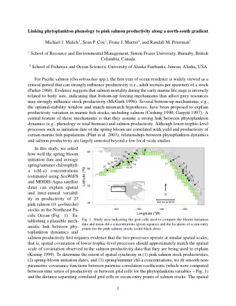
Linking phytoplankton phenology to pink salmon productivity along a north-south gradient Michael Malick Simon Fraser University, BC, Canada Sean Cox, Randall Peterman, & Franz Mueter @michaelmalick

Bottom-up Control b 1999 1 0 ) B S S 8 Phytoplankton phenology / R 1981 ( x 6 e (Platt et al. 2003) d n 1998 i l a 4 v i v 1980 r 2000 u 2001 S 2 1979 , 1997 2 1 0 – 1 – 2 – 3 Anomalies in t he t iming o f spring blooms ( weeks ) 2

Bottom-up Control b 1999 1 0 ) B S S 8 Phytoplankton phenology / R 1981 ( x 6 e (Platt et al. 2003) d n 1998 i l a 4 v i v 1980 r 2000 u 2001 S 2 1979 , 1997 2 1 0 – 1 – 2 – 3 Anomalies in t he t iming o f spring blooms ( weeks ) 2 = 0.87; r 2.0 Mean resident fish yield p < 0.0001; (metric tons km ) = 11 -2 n Phytoplankton biomass (Ware and Thomson 2005) 1.0 0.0 0 2 4 6 2 -3 Mean chl-a concentration (mg m )

Bottom-up Control b 1999 1 0 ) B S S 8 Phytoplankton phenology / R 1981 ( x 6 e (Platt et al. 2003) d n 1998 i l a 4 v i v 1980 r 2000 u 2001 S 2 1979 , 1997 2 1 0 – 1 – 2 – 3 Anomalies in t he t iming o f spring blooms ( weeks ) 2 = 0.87; r 2.0 Mean resident fish yield p < 0.0001; (metric tons km ) = 11 -2 n Phytoplankton biomass (Ware and Thomson 2005) 1.0 0.0 0 2 4 6 2 -3 Mean chl-a concentration (mg m )

Bottom-up Control 3

Bottom-up Control Survival Marine growth 3

Research Question Do changes in coastal phytoplankton phenology or biomass significantly influence pink salmon productivity? 4

Spatial Covariation Alaska ● ● ● ● ● ● ● ● ● ● ● ● ● ● ● ● ● ● ● ● ● ● ● ● ● ● ● ● ● ● ● ● ● ● ● ● ● ● ● ● ● ● ● ●● ● ● ● ● ● ●● ● ● ● ● ● ● ● ● ● BC ● ● ● ● ● ● ● ● ● ● ● ● ● ● ● ● ● ● ● ● ● ● ● ● ● ● ● ● ● ● ● ● ● ● 5 (Pyper et al. 2001)

Spatial Covariation Alaska ● ● ● ● ● ● Does the extent of spatial covariation ● ● for phytoplankton phenology and ● ● ● ● ● ● ● ● ● ● ● ● ● ● ● ● biomass match pink salmon? ● ● ● ● ● ● ● ● ● ● ● ● ● ● ● ● ● ● ● ●● ● ● ● ● ● ●● ● ● ● ● ● ● ● ● ● BC ● ● ● ● ● ● ● ● ● ● ● ● ● ● ● ● ● ● ● ● ● ● ● ● ● ● ● ● ● ● ● ● ● ● 6 (Pyper et al. 2001)

Salmon Data 4 ● Productivity (R/S) ● ● ● ● 3 ● ● 2 ● ● ● ● 1 ● ● 0 1998 2000 2002 2004 2006 2008 2010 Year 7

Phytoplankton Data • Spring bloom initiation date 14 ● Spring bloom initiation ● 12 ● ● 10 ● 8 ● ● ● ● ● 6 ● ● ● 1998 2000 2002 2004 2006 2008 2010 Year 8

Phytoplankton Data • Spring bloom initiation date • Phytoplankton biomass (mg/m 3 ) 14 ● Spring bloom initiation ● 12 ● ● 10 ● 8 ● ● ● ● ● 6 ● ● ● 1998 2000 2002 2004 2006 2008 2010 Year May ● 8 Biomass (mg / m 3 ) ● 6 ● ● 4 ● ● ● ● ● ● 2 ● ● ● 8 1998 2000 2002 2004 2006 2008 2010 Year

Spatial Covariation Correlation 0 50% Correlation Scale Distance (km) 1. Calculate cross-correlations 2. Plot correlations as a function of geographic distance 3. Fit covariance function to scatterplot 4. Estimate 50% correlation scale 9

Hierarchical Models log e (R i,t /S i,t ) = α + a i - β i S i,t + δ X i,t+1 + d i X i,t+1 + ε i,t Regional ... Stock #1 Stock #2 Stock #27 2.5 ● ● ● 2.0 ● ● 2.0 2.0 ● ● ● ● ● ● ● 1.5 ● ● 1.5 ● ● ● 1.5 ● log(R/S) ● log(R/S) log(R/S) ● ● ● ● ● ● ● ● ● ● ● ● ● ● ● ● ● ● ● ● ● ● ● ● ● ● 1.0 1.0 ● ● ● 1.0 ● ● ● ● ● ● ● ● ● ● ● ● ● ● ● ● ● ● ● ● ● ● ● ● ● ● ● ● ● ● ● ● ● ● ● ● ● ● 0.5 ● ● ● ● ● ● ● 0.5 ● ● ● 0.5 ● ● ● ● ● ● ● ● ● ● ● ● ● ● ● ● ● ● ● ● ● 0.0 0.0 ● 0.0 ● ● ● ● ● − 0.5 ● ● ● ● − 0.5 ● ● ● − 0.5 ● 2 4 6 8 10 5 10 15 20 25 30 5 10 10 Spawners Spawners Spawners

Hierarchical Models log e (R i,t /S i,t ) = α + a i - β i S i,t + δ X i,t+1 + d i X i,t+1 + ε i,t Regional • Spring bloom initiation date • Phytoplankton biomass (July-September) ... Stock #1 Stock #2 Stock #27 2.5 ● ● ● 2.0 ● ● 2.0 2.0 ● ● ● ● ● ● ● 1.5 ● ● 1.5 ● ● ● 1.5 ● log(R/S) ● log(R/S) log(R/S) ● ● ● ● ● ● ● ● ● ● ● ● ● ● ● ● ● ● ● ● ● ● ● ● ● ● 1.0 1.0 ● ● ● 1.0 ● ● ● ● ● ● ● ● ● ● ● ● ● ● ● ● ● ● ● ● ● ● ● ● ● ● ● ● ● ● ● ● ● ● ● ● ● ● 0.5 ● ● ● ● ● ● ● 0.5 ● ● ● 0.5 ● ● ● ● ● ● ● ● ● ● ● ● ● ● ● ● ● ● ● ● ● 0.0 0.0 ● 0.0 ● ● ● ● ● − 0.5 ● ● ● ● − 0.5 ● ● ● − 0.5 ● 2 4 6 8 10 5 10 15 20 25 30 5 10 11 Spawners Spawners Spawners

Spatial Covariation 12

Pink Salmon Productivity 1.0 ● ● ● ● ● ● ● ● ● ● ● ● ● ● ● ● ● ● ● ● ● ● ● ● Correlation coefficient ● ● ● ● ● ● ● ● ● ● ● ● ● ● ● ● ● Covariance function ● ● ● ● ● ● ● 0.5 ● ● ● ● ● ● ● ● ● ● ● ● ● ● ● ● ● ● ● ● ● ● ● ● ● ● ● ● ● ● ● ● ● ● ● ● ● ● ● ● ● ● ● ● ● ● ● ● ● ● ● ● ● ● ● ● ● ● ● ● ● ● ● ● ● ● ● ● ● ● ● ● ● ● ● ● ● ● ● ● ● ● ● ● ● ● ● ● ● ● ● ● ● ● ● ● ● ● ● ● ● ● ● ● ● ● ● ● ● ● ● ● ● ● ● ● ● ● ● ● ● ● ● ● ● ● ● ● ● ● ● ● ● ● ● ● ● ● ● ● ● ● 0.0 ● ● ● ● ● ● ● ● ● ● ● ● ● ● ● ● ● ● ● ● ● ● ● ● ● ● ● ● ● ● ● ● ● ● ● ● ● ● ● ● ● ● ● ● ● ● ● ● ● ● ● ● ● ● ● ● ● ● ● ● ● ● ● 50% correlation scale ● ● ● ● ● ● ● ● ● ● ● ● ● ● ● ● ● ● ● ● ● ● ● ● ● ● ● ● ● ● ● ● ● ● ● ● ● ● ● ● ● ● ● ● ● ● ● ● ● ● ● ● ● ● ● ● ● ● ● ● ● ● ● ● ● ● ● ● ● ● ● ● ● ● ● ● ● ● ● ● ● ● ● − 0.5 ● ● ● ● ● ● ● ● ● ● ● ● ● ● ● ● 261 km (148-628 km) − 1.0 500 1000 1500 2000 2500 Distance (km) 13