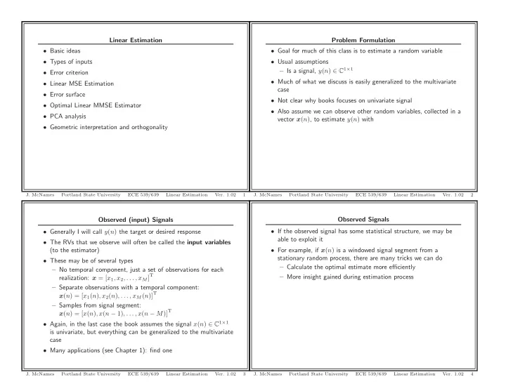
Linear Estimation Problem Formulation Basic ideas Goal for much of - PowerPoint PPT Presentation

Linear Estimation Problem Formulation • Basic ideas • Goal for much of this class is to estimate a random variable • Types of inputs • Usual assumptions – Is a signal, y ( n ) ∈ C 1 × 1 • Error criterion • Much of what we discuss is easily generalized to the multivariate • Linear MSE Estimation case • Error surface • Not clear why books focuses on univariate signal • Optimal Linear MMSE Estimator • Also assume we can observe other random variables, collected in a • PCA analysis vector x ( n ) , to estimate y ( n ) with • Geometric interpretation and orthogonality J. McNames Portland State University ECE 539/639 Linear Estimation Ver. 1.02 1 J. McNames Portland State University ECE 539/639 Linear Estimation Ver. 1.02 2 Observed (input) Signals Observed Signals • If the observed signal has some statistical structure, we may be • Generally I will call y ( n ) the target or desired response able to exploit it • The RVs that we observe will often be called the input variables (to the estimator) • For example, if x ( n ) is a windowed signal segment from a stationary random process, there are many tricks we can do • These may be of several types – Calculate the optimal estimate more efficiently – No temporal component, just a set of observations for each realization: x = [ x 1 , x 2 , . . . , x M ] T – More insight gained during estimation process – Separate observations with a temporal component: x ( n ) = [ x 1 ( n ) , x 2 ( n ) , . . . , x M ( n )] T – Samples from signal segment: x ( n ) = [ x ( n ) , x ( n − 1) , . . . , x ( n − M )] T • Again, in the last case the book assumes the signal x ( n ) ∈ C 1 × 1 is univariate, but everything can be generalized to the multivariate case • Many applications (see Chapter 1): find one J. McNames Portland State University ECE 539/639 Linear Estimation Ver. 1.02 3 J. McNames Portland State University ECE 539/639 Linear Estimation Ver. 1.02 4

Estimation Problem Error Signal Given a random vector x ( n ) ∈ C M × 1 , determine an estimate ˆ y ( n ) y ( n ) � y ( n ) − ˆ y ( n ) � e ( n ) ˜ using a “rule” • We want ˆ y ( n ) to be as close to y ( n ) as possible y ( n ) � h [ x ( n )] ˆ • In order to find the “optimal” estimator, we must have a • The “rule” h [ x ( n )] is called the estimator definition of optimality • In general it is (could be) a nonlinear function • Most definitions are functions of the error signal , e ( n ) • If x ( n ) = [ x ( n ) , x ( n − 1) , . . . , x ( n − M )] T , the estimator is called • They are not equivalent, in general a discrete-time filter • Let P denote the performance criterion • The estimator could be • Also called the performance metric or cost function – Linear or nonlinear – Time-invariant or time-varying, h n [ x ( n )] • May wish to maximize or minimize depending on the definition – FIR or IIR J. McNames Portland State University ECE 539/639 Linear Estimation Ver. 1.02 5 J. McNames Portland State University ECE 539/639 Linear Estimation Ver. 1.02 6 Ensemble versus Realizations Estimators Optimum Estimator Design • Fundamentally, the book discusses two approaches to estimation 1. Select a structure for the estimator (usually parametric) • Ensemble Performance Metrics 2. Select a performance criterion – P is a function of the joint distribution of [ y ( n ) , x ( n ) T ] 3. Optimize the estimator (solve for the best parameter values) – Estimator performs well on the ensemble 4. Assess the estimator performance – Chapters 6 and 7 – Example: Minimum Mean Square Error (MMSE) • Realization Performance Metrics – P is a function of observed data (a realization) – Estimator performs well on that data set – Chapters 8 and 9 – Example: Least square error (LSE) • The two approaches are closely related J. McNames Portland State University ECE 539/639 Linear Estimation Ver. 1.02 7 J. McNames Portland State University ECE 539/639 Linear Estimation Ver. 1.02 8

Selection of Performance Criterion Error Measures • It is often difficult to express subjective criteria (e.g., health, Various Measures of Model Performance 9 sound quality, image quality) mathematically Squared Error 8 • This is where your judgement, experience are required to make a Absolute Error design decision that is suited to your application Root Absolute Error 7 • Fundamental tradeoff: tractability of the solution versus accuracy 6 Error Measures of subjective quality 5 • Is usually a function of the estimation error 4 • Often has even symmetry: p [ e ( n )] = p [ e ( − n )] 3 – Positive errors are equally harmful as negative errors 2 1 0 −3 −2 −1 0 1 2 3 Error: e ( n ) = y ( n ) − ˆ y ( n ) J. McNames Portland State University ECE 539/639 Linear Estimation Ver. 1.02 9 J. McNames Portland State University ECE 539/639 Linear Estimation Ver. 1.02 10 Selection of Performance Criterion Statistical Signal Processing Scope • If approximation to subjective criteria is irrelevant or unimportant, • Much of the known theory is limited to two other factors motivate the choice – MSE or ASE / SSE performance metrics 1. Sensitivity to outliers – Linear estimators 2. Mathematical tractability • Why? • Error measures like median absolute error and mean absolute error – Thorough and elegant optimal results are known are more tolerant of outliers (given less relative weight) – Only requires knowledge of second-order moments, which can • Mean squared error is usually the most mathematically tractable be estimated (ECE 5/638) – Differentiable – Many of the other cases are generalizations of the linear case – Only a function of the second order moments of e ( n ) : doesn’t • This is a critical foundation for a career in signal processing require knowledge of the distribution or pdf f e ( n ) ( e ) – Is same as maximum likelihood estimate when e ( n ) is Gaussian – Often, it works J. McNames Portland State University ECE 539/639 Linear Estimation Ver. 1.02 11 J. McNames Portland State University ECE 539/639 Linear Estimation Ver. 1.02 12

Linear MSE Estimation Notation I believe the book chose the linear estimator to use the complex M � y ( n ) � c ( n ) H x = c ∗ P ( c ( n )) � E[ | e ( n ) | 2 ] conjugate of the coefficients, ˆ k ( n ) x k ( n ) k =1 M � c H • Design goal: design a linear estimator of y ( n ) that minimizes the y ( n ) = ˆ k x k ( n ) MSE k =1 • Equivalent to solving for the model coefficients c such that the so that this could be defined as an inner product of the parameter or coefficient vector c ∈ C M × 1 and the input data vector MSE is minimized x ( n ) ∈ C M × 1 as • We assume that the RVs { y ( n ) , x ( n ) T } are realizations of a stochastic process M � • If jointly nonstationary, the optimal coefficients are time-varying, c H x = c k x k = c k · x k = � c , x � c ( n ) k =1 • The time index will often be dropped to simplify notation The parameter vector that minimizes the MSE , denoted as c o is called M the linear MMSE ( LMMSE ) estimator � y ( n ) � c H x = c H P ( c ) � E[ | e ( n ) | 2 ] ˆ k x k ( n ) y o is called the LMMSE estimate ˆ k =1 J. McNames Portland State University ECE 539/639 Linear Estimation Ver. 1.02 13 J. McNames Portland State University ECE 539/639 Linear Estimation Ver. 1.02 14 Zero Mean Assumption Error Performance Surface The error performance surface is simply the multivariate error criterion All RVs are assumed to have zero mean expressed as a function of the parameter vector • Greatly simplifies the math P ( c ) = E[ | e | 2 ] • Means that all covariances are simply correlations ( y − c H x ))( y ∗ − x H c ) � � = E • In practice, is enforced by removing the mean and/or trend = E[ | y | 2 ] − c H E[ x y ∗ ] − E[ y x H ] c + c H E[ xx H ] c – Subtract the sample average and assume statistical impact is negligible = P y − c H d − d H c + c H Rc – Highpass filter, but watch for edge effects where – First order difference � E[ | y | 2 ] M × M � E[ xx H ] M × 1 � E[ x y ∗ ] – Other (detrend) P y d R 1 × 1 • This is a gotcha, so watch this carefully You should be able to show that R is Hermitian and nonnegative definite. In virtually all practical applications, it is positive definite and invertible. J. McNames Portland State University ECE 539/639 Linear Estimation Ver. 1.02 15 J. McNames Portland State University ECE 539/639 Linear Estimation Ver. 1.02 16

Error Performance Surface Example 1: Error Performance Surface P ( c ) = P y − c H d − d H c + c H Rc Plot the error surface for the following covariance matrices. What is the optimal solution? • P ( c ) is called the error performance surface • It is a quadratic function of the parameter vector c • If R is positive definite, it is strictly convex with a single minimum at the optimal solution c o • Can think of as a quadratic bowl in an M dimensional space • Our goal is to find the bottom of the bowl J. McNames Portland State University ECE 539/639 Linear Estimation Ver. 1.02 17 J. McNames Portland State University ECE 539/639 Linear Estimation Ver. 1.02 18 Example 1: Error Performance Surface Example 1: Error Performance Surface 6 50 40 50 5 30 40 40 4 20 3 10 30 30 2 0 c 1 1 −10 20 20 −20 0 6 10 10 −1 4 −2 2 0 0 0 −3 −2 c 1 6 4 −2 0 2 4 6 2 0 −2 c 2 c 2 J. McNames Portland State University ECE 539/639 Linear Estimation Ver. 1.02 19 J. McNames Portland State University ECE 539/639 Linear Estimation Ver. 1.02 20