Lexical Semantics (Following slides are modified from Prof. Claire - PowerPoint PPT Presentation
Lexical Semantics (Following slides are modified from Prof. Claire Cardies slides.) Introduction to lexical semantics Lexical semantics is the study of the systematic meaning-related connections among words and the internal
Lexical Semantics (Following slides are modified from Prof. Claire Cardie’s slides.)
Introduction to lexical semantics Lexical semantics is the study of the systematic meaning-related connections among words and the internal meaning-related structure of each word Lexeme an individual entry in the lexicon a pairing of a particular orthographic and phonological form with some form of symbolic meaning representation Sense : the lexeme’s meaning component Lexicon: a finite list of lexemes
Dictionary entries right adj. left adj. red n. blood n.
Dictionary entries right adj. located nearer the right hand esp. being on the right when facing the same direction as the observer. left adj. located nearer to this side of the body than the right . red n. blood n.
Dictionary entries right adj. located nearer the right hand esp. being on the right when facing the same direction as the observer. left adj. located nearer to this side of the body than the right . red n. the color of blood or a ruby. blood n. the red liquid that circulates in the heart, arteries and veins of animals.
Lexical semantic relations: Homonymy Homonyms : words that have the same form and unrelated meanings The bank 1 had been offering 8 billion pounds in 91-day bills. As agriculture burgeons on the east bank 2 , the river will shrink even more. Homophones : distinct lexemes with a shared pronunciation E.g. would and wood , see and sea. Homographs : identical orthographic forms, different pronunciations, and unrelated meanings The fisherman was fly-casting for bass rather than trout. I am looking for headphones with amazing bass .
Lexical semantic relations: Polysemy Polysemy: the phenomenon of multiple related meanings within a single lexeme bank: financial institution as corporation bank: a building housing such an institution Homonyms (disconnected meanings) bank: financial institution bank: sloping land next to a river Distinguishing homonymy from polysemy is not always easy. Decision is based on: Etymology: history of the lexemes in question Intuition of native speakers
Lexical semantic relations: Synonymy Lexemes with the same meaning Invoke the notion of substitutability Two lexemes will be considered synonyms if they can be substituted for one another in a sentence without changing the meaning or acceptability of the sentence How big is that plane? Would I be flying on a large or small plane? Miss Nelson, for instance, became a kind of big sister to Mrs. Van Tassel’s son, Benjamin. We frustrate ‘ em and frustrate ‘ em, and pretty soon they make a big mistake.
Word sense disambiguation (WSD) Given a fixed set of senses associated with a lexical item, determine which of them applies to a particular instance of the lexical item Fundamental question to many NLP applications. Spelling correction Speech recognition Text-to-speech Information retrieval
WordNet (Following slides are modified from Prof. Claire Cardie’s slides.)
WordNet Handcrafted database of lexical relations Separate databases: nouns; verbs; adjectives and adverbs Each database is a set of lexical entries (according to unique orthographic forms) Set of senses associated with each entry
WordNet Developed by famous cognitive psychologist George Miller and a team at Princeton University. Try WordNet online at http://wordnetweb.princeton.edu/perl/webwn How many different meanings for “eat”? How many different meanings for “dog”?
Sample entry
WordNet Synset Synset == Synonym Set Synset is defined by a set of words Each synset represents a different “sense” of a word Consider synset == sense Which would be bigger? # of unique words V.S # of unique synsets
Statistics POS Unique Synsets Total Strings word+sense pairs Noun 117798 82115 146312 Verb 11529 13767 25047 Adj 21479 18156 30002 Adv 4481 3621 5580 Totals 155287 11765 206941
More WordNet Statistics Avg Polysemy w/o monosemous words Part-of-speech Avg Polysemy Noun 1.24 2.79 Verb 2.17 3.57 Adjective 1.40 2.71 Adverb 1.25 2.50
Distribution of senses Zipf distribution of senses
WordNet relations Nouns Verbs Adjectives/adverbs
Selectional Preference
Selectional Restrictions & Selectional Preferences I want to eat someplace that’s close to school. => “eat” is intransitive I want to eat Malaysian food. => “eat” is transitive “eat” expects its object to be edible. What about the subject of “eat”?
Selectional Restrictions & Selectional Preferences What are selectional restrictions (or selectional preferences) of… “imagine” “ diagonalize ” “odorless” Some words have stronger selectional preferences than others. How can we quantify the strength of selectional preferences?
Selectional Preference Strength P(c) := the distribution of semantic class ‘c’ P(c|v ) := the distribution of semantic class ‘c’ of the object of the given verb ‘v’ What does it mean if P(c) = P(c|v) ? What does it mean if P(c) is very different from P(c|v) ? The difference between distributions can be measured by Kullback-Leibler divergence (KL divergence) D ( P jj Q ) = P x P ( x ) log P ( x ) Q ( x )
Selectional Preference Strength Selectional preference of ‘v’ S R ( v ) := D ( P ( c j v ) jj P ( c )) X P ( c j v ) logP ( c j v ) = P ( c ) c Selectional association of ‘v’ and ‘c’ S R ( v ) P ( c j v ) logP ( c j v ) 1 A R ( v; c ) = P ( c ) The difference between distributions can be measured by Kullback-Leibler divergence (KL divergence) D ( P jj Q ) = P x P ( x ) log P ( x ) Q ( x )
Selectional Association Selectional association of ‘v’ and ‘c’ S R ( v ) P ( c j v ) logP ( c j v ) 1 A R ( v; c ) = P ( c )
Remember Pseudowords for WSD? Artificial words created by concatenation of two randomly chosen words E.g. “banana” + “door” => “banana - door” Pseudowords can generate training and test data for WSD automatically. How? Issues with pseudowords?
Pseudowords for Selectional Preference?
Word Similarity
Word Similarity Thesaurus Methods Distributional Methods
Word Similarity: Thesaurus Methods Path-length based similarity pathlen(nickel, coin) = 1 pathlen(nickel, money) = 5
Word Similarity: Thesaurus Methods pathlen(x 1 , x 2 ) is the shortest path between x 1 and X 2 Similarity between two senses --- s 1 and s 2 : sim path ( s 1 ;s 2 ) = ¡ log pathlen( s 1 ;s 2 ) Similarity between two words --- w 1 and w 2 ? wordsim( w 1 ; w 2 ) = max s 1 2 senses ( w 1 ) sim( s 1 ;s 2 ) s 2 2 senses ( w 2 )
Word Similarity: Thesaurus Methods Problems? Path-length based similarit pathlen(nickel, coin) = 1 pathlen(nickel, money) = 5
Information-content based word-similarity P(c) := the probability that a randomly selected word is an instance of concept ‘c’ P w 2 words ( c ) count ( w ) P ( c ) = N IC(c) := Information Content IC ( c ) := ¡ log P ( c ) LCS(c 1 , c 2 ) = the lowest common subsumer sim resnik ( c 1 ;c 2 ) = ¡ log P (LCS( c 1 ;c 2 ))
Examples of p(c)
Thesaurus-based similarity measures
Word Similarity Thesaurus Methods Distributional Methods
Distributional Word Similarity A bottle of tezguino is on the table. Tezguino makes you drunk. We make tezguino out of corn. Tezguino, beer, liquor, tequila, etc share contextual features such as Occurs before ‘drunk’ Occurs after ‘bottle’ Is the direct object of ‘likes’
Distributional Word Similarity Co-occurrence vectors
Distributional Word Similarity Co-occurrence vectors with grammatical relations I discovered dried tangerines discover (subject I) I (subj-of discover) tangerine (obj-of discover) tangerine (adj-mod dried) dried (adj-mod-of tangerine)
Distributional Word Similarity
Examples of PMI scores
Distributional Word Similarity Problems with Thesaurus-based methods? Some languages lack such resources Thesauruses often lack new words and domain-specific words Distributional methods can be used for Automatic thesaurus generation Augmenting existing thesauruses, e.g., WordNet
Vector Space Models for word meaning (Following slides are modified from Prof. Katrin Erk’s slides.)
Geometric interpretation of lists of feature/value pairs In cognitive science: representation of a concept through a list of feature/value pairs Geometric interpretation: Consider each feature as a dimension Consider each value as the coordinate on that dimension Then a list of feature-value pairs can be viewed as a point in “space” Example color represented through dimensions (1) brightness, (2) hue, (3) saturation
Recommend
More recommend
Explore More Topics
Stay informed with curated content and fresh updates.
