Lecture on Stochastic Differential Equations Erik Lindstrm - PowerPoint PPT Presentation

Lecture on Stochastic Differential Equations Erik Lindström

Motivation than discrete time models, at least if you have a background in science or engineering. It is often argued that continuous time models need fewer parameters compared to discrete time models, as the parameters often can be given an interpretation. Consistent with option valuation due to path wise properties. Integration between time scales (e.g. irregularly sampled data) Heteroscedasticity is easily integrated into the models. ◮ Continuous time models are more 'interpretable'

Motivation than discrete time models, at least if you have a background in science or engineering. need fewer parameters compared to discrete time models, as the parameters often can be given an interpretation. Consistent with option valuation due to path wise properties. Integration between time scales (e.g. irregularly sampled data) Heteroscedasticity is easily integrated into the models. ◮ Continuous time models are more 'interpretable' ◮ It is often argued that continuous time models

Motivation than discrete time models, at least if you have a background in science or engineering. need fewer parameters compared to discrete time models, as the parameters often can be given an interpretation. wise properties. Integration between time scales (e.g. irregularly sampled data) Heteroscedasticity is easily integrated into the models. ◮ Continuous time models are more 'interpretable' ◮ It is often argued that continuous time models ◮ Consistent with option valuation due to path

Motivation than discrete time models, at least if you have a background in science or engineering. need fewer parameters compared to discrete time models, as the parameters often can be given an interpretation. wise properties. sampled data) Heteroscedasticity is easily integrated into the models. ◮ Continuous time models are more 'interpretable' ◮ It is often argued that continuous time models ◮ Consistent with option valuation due to path ◮ Integration between time scales (e.g. irregularly

Motivation than discrete time models, at least if you have a background in science or engineering. need fewer parameters compared to discrete time models, as the parameters often can be given an interpretation. wise properties. sampled data) models. ◮ Continuous time models are more 'interpretable' ◮ It is often argued that continuous time models ◮ Consistent with option valuation due to path ◮ Integration between time scales (e.g. irregularly ◮ Heteroscedasticity is easily integrated into the

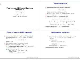
d t t d t t ODEs in physics d S noise r d S CAPM t S t , cf. RCAR noise Stock Physics is often modelled as (a system of) ordinary d B Bond Similar models are found in finance (1) d X differential equations t S t d t ( t ) = µ ( X ( t )) d t ( t ) = rB ( t )

d t t ODEs in physics Stock noise r d S CAPM d S t S t Physics is often modelled as (a system of) ordinary d B Bond Similar models are found in finance (1) d X differential equations d t ( t ) = µ ( X ( t )) d t ( t ) = rB ( t ) d t ( t ) = ( µ + “ noise ′′ ( t )) S ( t ) , cf. RCAR

ODEs in physics Physics is often modelled as (a system of) ordinary differential equations d X (1) Similar models are found in finance Bond d B Stock d S CAPM d S d t ( t ) = µ ( X ( t )) d t ( t ) = rB ( t ) d t ( t ) = ( µ + “ noise ′′ ( t )) S ( t ) , cf. RCAR d t ( t ) = ( r + βσ + σ “ noise ′′ ( t )) S ( t )

1 Y n 1 1 Noise processes N t n N t Note that N t n Compound Poisson process S t The noise process should ideally be the time t Poisson process N t , or N t Brownian motion W t time processes (see Chapter 7.5) Examples of continuous derivative of random walk. Lévy process L t

1 Y n 1 1 Noise processes The noise process should ideally be the time derivative of random walk. Examples of continuous time processes (see Chapter 7.5) Poisson process N t , or N t t Compound Poisson process S t N t n Note that N t N t n Lévy process L t ◮ Brownian motion W ( t )

1 Y n 1 1 Noise processes The noise process should ideally be the time derivative of random walk. Examples of continuous time processes (see Chapter 7.5) Compound Poisson process S t N t n Note that N t N t n Lévy process L t ◮ Brownian motion W ( t ) ◮ Poisson process N ( t ) , or ( N ( t ) − λ t )

1 1 Noise processes The noise process should ideally be the time derivative of random walk. Examples of continuous time processes (see Chapter 7.5) Note that N t N t n Lévy process L t ◮ Brownian motion W ( t ) ◮ Poisson process N ( t ) , or ( N ( t ) − λ t ) ◮ Compound Poisson process S ( t ) = ∑ N ( t ) n = 1 Y n

Noise processes The noise process should ideally be the time derivative of random walk. Examples of continuous time processes (see Chapter 7.5) Lévy process L t ◮ Brownian motion W ( t ) ◮ Poisson process N ( t ) , or ( N ( t ) − λ t ) ◮ Compound Poisson process S ( t ) = ∑ N ( t ) n = 1 Y n ◮ Note that N ( t ) = ∑ N ( t ) n = 1 1

Noise processes The noise process should ideally be the time derivative of random walk. Examples of continuous time processes (see Chapter 7.5) ◮ Brownian motion W ( t ) ◮ Poisson process N ( t ) , or ( N ( t ) − λ t ) ◮ Compound Poisson process S ( t ) = ∑ N ( t ) n = 1 Y n ◮ Note that N ( t ) = ∑ N ( t ) n = 1 1 ◮ Lévy process L ( t )

Wiener process aka Standard Brownian Motion A processes satisfying the following conditions is a Standard Brownian Motion ◮ X ( 0 ) = 0 with probability 1. ◮ The increments W ( u ) − W ( t ) , W ( s ) − W ( 0 ) with u > t ≥ s > 0 are independent. ◮ The increment W ( t ) − W ( s ) ∼ N ( 0 , t − s ) ◮ The process has continuous trajectories.

Time derivative of the Wiener process Study the object h (2) The limit does not converge in mean square sense! ξ h = W ( t + h ) − W ( t ) (Think d W ( t ) / d t = lim h → 0 ξ h ). Compute ◮ E [ ξ h ] ◮ Var [ ξ h ]

Time derivative of the Wiener process Study the object h (2) The limit does not converge in mean square sense! ξ h = W ( t + h ) − W ( t ) (Think d W ( t ) / d t = lim h → 0 ξ h ). Compute ◮ E [ ξ h ] ◮ Var [ ξ h ]

Re-interpreting ODEs 0 (5) X s d s 0 t X 0 X t d X s t In physics, or actually (4) X t d t d X t really means (3) d X NOTE: No derivatives needed! d t ( t ) = µ ( X ( t ))

Re-interpreting ODEs 0 (5) X s d s 0 t X 0 X t d X s t In physics, or actually (4) really means (3) d X NOTE: No derivatives needed! d t ( t ) = µ ( X ( t )) d X ( t ) = µ ( X ( t )) d t

Re-interpreting ODEs (4) (5) 0 0 In physics, or actually really means (3) d X NOTE: No derivatives needed! d t ( t ) = µ ( X ( t )) d X ( t ) = µ ( X ( t )) d t ∫ t ∫ t d X ( s ) = X ( t ) − X ( 0 ) = µ ( X ( s )) d s

Stochastic differential equations d s X s d W s X s d s X 0 X t Stochastic Differential Equations as The mathematically correct approach is to define (8) 0 Interpret (7) (9) as d X 0 (6) µ ( X ( t )) + “ noise ′′ ( t ) ( ) d t = ∫ t µ ( X ( s )) + “ noise ′′ ( s ) ( ) X ( t ) − X ( 0 ) ≈ ∫ t ∫ ≈ µ ( X ( s )) d s + σ ( X ( s )) d v d s d s

Stochastic differential equations 0 Stochastic Differential Equations as The mathematically correct approach is to define (8) 0 Interpret d s (7) (9) as (6) d X µ ( X ( t )) + “ noise ′′ ( t ) ( ) d t = ∫ t µ ( X ( s )) + “ noise ′′ ( s ) ( ) X ( t ) − X ( 0 ) ≈ ∫ t ∫ ≈ µ ( X ( s )) d s + σ ( X ( s )) d v d s d s ∫ ∫ X ( t ) − X ( 0 ) = µ ( X ( s )) d s + σ ( X ( s )) d W ( s )

Integrals The (10) integral is an ordinary Riemann integral, whereas the X s d W s (11) integral is an Ito integral. ∫ µ ( X ( s )) d s

Integrals The (10) integral is an ordinary Riemann integral,whereas the (11) o integral. ∫ µ ( X ( s )) d s ∫ σ ( X ( s )) d W ( s ) integral is an It ¯

sense. o integral tend to zero. The limit is computed in L 2 o integral is defined (for a piece-wise constant constant functions, while letting the discretization b General functions are approximated by piece-wise a e It ¯ The It ¯ integrand σ ( s , ω ) ) as n − 1 ∫ ∑ σ ( s , ω ) dW ( s ) = σ ( t k , ω )( W ( t k + 1 ) − W ( t k )) . (12) k = 0

o integral o integral is defined (for a piece-wise constant b a General functions are approximated by piece-wise constant functions, while letting the discretization e It ¯ The It ¯ integrand σ ( s , ω ) ) as n − 1 ∫ ∑ σ ( s , ω ) dW ( s ) = σ ( t k , ω )( W ( t k + 1 ) − W ( t k )) . (12) k = 0 tend to zero. The limit is computed in L 2 ( P ) sense.

Properties 0 (14) X s E E n 1 k t k d W u W t k 1 W t k t k s X s s u Stochastic integrals are martingales. E X s Proof: E X t E s X t X t s (13) X s (15) Definition: A stochastic process { X ( t ) , t ≥ 0 } is called a martingale with respect to a filtration {F ( t ) } t ≥ 0 if ◮ X ( t ) is F ( t ) -measurable for all t ◮ E [ | X ( t ) | ] < ∞ for all t , and ◮ E [ X ( t ) |F ( s )] = X ( s ) for all s ≤ t .