Lecture 8: F -Test for Nested Linear Models Zhenke Wu Department of - PowerPoint PPT Presentation
Lecture 8: F -Test for Nested Linear Models Zhenke Wu Department of Biostatistics Johns Hopkins Bloomberg School of Public Health zhwu@jhu.edu http://zhenkewu.com 11 February, 2016 Lecture 8 140.653 Methods in Biostatistics 1 Lecture 7
Lecture 8: F -Test for Nested Linear Models Zhenke Wu Department of Biostatistics Johns Hopkins Bloomberg School of Public Health zhwu@jhu.edu http://zhenkewu.com 11 February, 2016 Lecture 8 140.653 Methods in Biostatistics 1
Lecture 7 Main Points Again Constructing F -distribution: independently distributed ◮ Y i Gaussian ( µ i , σ 2 ∼ i ) iid ◮ Z i = Y i − µ i ; Z i ∼ Gaussian (0 , 1) σ i ◮ Define quadratic forms Q 1 = Z 2 1 + · · · + Z 2 n 1 and Q 2 = Z 2 n 1 +1 + · · · + Z 2 n 1 + n 2 ◮ Q 1 ∼ χ 2 n 1 with mean n 1 and variance 2 n 1 ◮ Q 2 ∼ χ 2 n 2 with mean n 2 and variance 2 n 2 ◮ Q 1 is independent of Q 2 ◮ F n 1 , n 2 = Q 1 / n 1 Q 2 / n 2 ∼ F ( n 1 , n 2 ) ( F -distribution with n 1 and n 2 degrees of freedom; “ F ” for Sir R.A. Fisher) Lecture 8 140.653 Methods in Biostatistics 2
Lecture 7 Main Points Again (continued) ◮ Data: ◮ n observations; p + s covariates ◮ continuous outcome Y i , measured with error ◮ covariates: X i = ( X i 1 , . . . , X ip , X i , p +1 , . . . , X i , p + s ) ⊤ , for i = 1 , . . . , n ◮ Question: In light of data, can we use a simpler linear model nested within a complex one? ◮ Hypothesis testing: (a) Null model: Y ∼ Gaussian n ( X N β N , σ 2 I n ) ◮ X N : design matrix n × ( p + 1) obtained by stacking observations X i ◮ First p (transformed) covariates and 1 intercept ◮ Regression coefficients: β N = ( β 0 , β 1 , . . . , β p ) ⊤ ◮ Standard deviation of measurement errors: σ (b) Extended model: Y ∼ Gaussian n ( X E β E , σ 2 I n ) ◮ X E : design matrix with intercept+ p + s covariates ◮ β E = ( β ⊤ N , β p +1 , . . . , β p + s ) ⊤ Null model: H 0 : β p +1 = β p +2 = · · · = β p + s = 0 ◮ Lecture 8 140.653 Methods in Biostatistics 3
Lecture 7 Main Points Again (continued) Null model: H 0 : β p +1 = β p +2 = · · · = β p + s = 0 Let β [ p +] = ( β p +1 , · · · , β p + s ) ⊤ ◮ Rationale of the F -Test ◮ If H 0 is true, estimates � β p +1 , · · · , � β p + s should all be close to 0 ◮ Reject H 0 if these estimates are sufficiently different from 0s. ◮ However, not every � β p + j , j = 1 , . . . , s , should be treated the same; they have different precisions ◮ Use a quadratic term to measure their joint differences from 0, taking account of different precisions: � � − 1 � � Var E [ � β ⊤ β [ p +] ] β [ p +] (1) [ p +] ◮ Var E [ � β [ p +] ] = σ 2 A ( X ⊤ E X E ) − 1 A ⊤ , where A = [ 0 s × ( p +1) , I s × s ] ◮ Estimate σ 2 by RSS E / ( n − p − s − 1); RSS for ”residual sum of squares” Lecture 8 140.653 Methods in Biostatistics 4
Lecture 7 Main Points Again (continued) ◮ ( RSS N − RSS E ) / s F = (2) RSS E / ( n − p − s − 1) ◮ F ( s , n − p − s − 1): F -distribution with s and n − p − s − 1 degrees of freedom N X N ) − 1 X N ; “ H ” for hat matrix, ◮ RSS N = Y ′ ( I − H N ) Y ; H N = X N ( X ′ or projector E X E ) − 1 X E ◮ RSS E = Y ′ ( I − H E ) Y ; H E = X E ( X ′ ◮ ( RSS N − RSS E ) /σ 2 ∼ χ 2 s and RSS E /σ 2 ∼ χ 2 n − p − s − 1 ; they are independent [Proof]: ◮ Algebraic: The former is a function of � β E , which is independent of RSS E ] ◮ Geometric: Squared lengths of orthogonal vectors Lecture 8 140.653 Methods in Biostatistics 5
Geometric Interpretation: Projection ◮ � Y N = H N Y : fitted means under the null model ◮ � Y E = H E Y : fitted means under the extended model R > N R N Y X p +1 , · · · , X p + s ˆ Y E R > E R E ˆ Y N 1 , X 1 , . . . , X p R > N R N − R > E R E Model Space Lecture 8 140.653 Methods in Biostatistics 6
Analysis of Variance (ANOVA) for Regression Table: ANOVA for Regression Resudial Residual Sum Residual Model df df of Squares (RSS) Mean Square R ′ N R N RSS N = R ′ n − p − 1 = S 2 Null p + 1 n − p − 1 N R N N R ′ E R E RSS E = R ′ n − p − s − 1 = S 2 Extended p + s + 1 n − p − s − 1 E R E E R ′ N R N − R ′ E R E ( R ′ N R N − R ′ Change − s E R E ) s s = R ′ N R N − R ′ E R E ( R ′ N R N − R ′ E R E ) / s ◮ F s , n − p − s − 1 = R ′ E R E / ( n − p − s − 1) ◮ Reject H 0 if F > F 1 − α ( s , n − p − s − 1) , e.g., α = 0 . 05 � �� � (1 − α %) percentile of the F distribution Lecture 8 140.653 Methods in Biostatistics 7
Some Quick Facts about F -distribution Special cases of F ( n 1 , n 2 ) ◮ n 2 → ∞ : in probability ◮ Q 2 / n 2 − → constant in distribution ◮ For a fixed n 1 , F n 1 , n 2 Q 1 / n 1 ∼ χ 2 n 1 / n 1 as n 2 approaches − → infinity ◮ Or equivalently n 1 F n 1 , ∞ ∼ χ 2 n 1 ◮ If s = 1: β p +1 ) 2 for testing the null model ◮ The F -statistic equals ( � β p +1 / se � H 0 : β p +1 = 0 ◮ Under H 0 , it is distributed as F (1 , n − p − 2) ◮ Approximately distributed as χ 2 1 / 1 when n >> p (therefore 3 . 84 is the critical value at the 0 . 05 level) Lecture 8 140.653 Methods in Biostatistics 8
F -Table For F distribution with denominator df 2 = 1 , 2, the 0 . 95 percentile increases with df 1 ; for df 2 > 2, the percentile decreases with df 1 . df 2 \ df 1 1 2 3 10 100 1 161.45 199.50 215.71 241.88 253.04 2 18.51 19.00 19.16 19.40 19.49 3 10.13 9.55 9.28 8.79 8.55 100 3.94 3.09 2.70 1.93 1.39 1000 3.85 3.00 2.61 1.84 1.26 ∞ 3.84 3.00 2.60 1.83 1.24 Table: 95% quantiles for F-distribution with degrees of freedom df 1 and df 2 . Lecture 8 140.653 Methods in Biostatistics 9
Lecture 8 F -Table df 2 df 2 2e+08 1000 100 3 2 1 0.0 0.4 0.8 0.0 0.4 0.8 0.0 0.4 0.8 0.0 0.4 0.8 0.0 0.4 0.8 0.0 0.4 0.8 Figure: Density functions for F distributions; Red lines for 95% quantiles 0 0 0 0 0 0 2 2 2 2 5 50 100 4 4 4 4 10 1 15 150 6 6 6 6 200 8 8 8 8 20 250 10 10 10 10 25 0 0 0 0 0 0 50 2 2 2 2 5 10 100 4 4 4 4 2 150 6 6 6 6 15 20 200 8 8 8 8 140.653 Methods in Biostatistics 10 10 10 10 25 250 0 0 0 0 0 0 50 2 2 2 2 5 100 4 4 4 4 10 df 1 df 1 3 15 150 6 6 6 6 20 200 8 8 8 8 250 10 10 10 10 25 0 0 0 0 0 0 2 2 2 2 5 50 10 100 4 4 4 4 5 150 6 6 6 6 15 200 8 8 8 8 20 10 10 10 10 25 250 0 0 0 0 0 0 50 2 2 2 2 5 100 4 4 4 4 10 6 150 6 6 6 6 15 20 200 8 8 8 8 250 10 10 10 10 25 10
Example ◮ Data: National Medical Expenditure Survey (NMES) ◮ Objective: To understand the relationship between medical expenditures and presence of a major smoking-caused disease among persons who are similar with respect to age, sex and SES ◮ Y i = log e ( total medical expenditure i + 1) ◮ X i 1 = age i − 65 years ◮ X i 2 = ♂ ◮ # of subjects : n = 4078 Lecture 8 140.653 Methods in Biostatistics 11
Example Table: NMES Fitted Models Model Design df Residual MS Resid. df A X 1 , X 2 3 1.521 4075 X 1 , ( X 1 − ( − 20) + , ( X 1 − 0) + ), X 2 B 5 1.518 4073 [ X 1 , ( X 1 − ( − 20) + , ( X 1 − 0) + )] ∗ X 2 C 8 1.514 4070 � �� � all interactions and main effects Lecture 8 140.653 Methods in Biostatistics 12
NMES Example: Question 1 Is average log medical expenditures roughly a linear function of age? ◮ Compare which two models? ◮ Calculate Residual Sum of Squares and Residual Mean Squares. ◮ Calculate F -statistic; What are the degrees of freedom for its distribution under the null? ◮ Compare it to the critical value at the 0 . 05 level Lecture 8 140.653 Methods in Biostatistics 13
NMES Example: Question 1 ◮ H 0 : Within a larger model B, model A is true (or state the scientific meaning, i.e., linearity in age). ◮ change in df ���� ( RSS N − RSS E ) / s F = (3) RSS E / ( n − p − s − 1) � �� � � �� � residual sum of squares residual df � �� � residual mean squares (1 . 521 × 4075 − 1 . 518 × 4073) / 2 = = 5 . 03 (4) 1 . 518 ◮ This statistic, under repeated sampling, has a F (2 , 4073) distribution, which is approximately χ 2 2 / 2 distributed. ◮ p-value: Pr ( χ 2 / 2 > 5 . 03) = 0 . 0065 by approximation or Pr ( F (2 , 4073) > 5 . 03) = 0 . 0066 without approximation. The approximation is good. ◮ Reject linearity in age. Lecture 8 140.653 Methods in Biostatistics 14
NMES Example: Question 2 (In-Class Exercise) ◮ Is the non-linear relationship of average log expenditure on age the same for ♂ and ♀ ? (Are there curves parallel?) ◮ Or equivalently, is the difference between average log medical expenditure for ♂ -vs- ♀ the same at all ages? Lecture 8 140.653 Methods in Biostatistics 15
NMES Example: Question 2 (In-Class Exercise) ◮ H 0 : Within a larger model C, model B is true (or equivalently state the scientific meaning, i.e., no interaction). ◮ (1 . 518 × 4073 − 1 . 514 × 4070) / 3 F = = 4 . 59 (5) 1 . 514 ◮ Under repeated sampling, it is F (3 , 4070) distributed. ◮ p-value Pr ( χ 2 3 / 3 > 4 . 59) = 0 . 0032 by approximation, or Pr ( F (3 , 4070) > 4 . 59) = 0 . 0033 without approximation. ◮ Reject no-interaction assumption Lecture 8 140.653 Methods in Biostatistics 16
Recommend
More recommend
Explore More Topics
Stay informed with curated content and fresh updates.
