Lecture 6 Geometric Transformations and Image Registration Lin - PowerPoint PPT Presentation

Lecture 6 Geometric Transformations and Image Registration Lin ZHANG, PhD School of Software Engineering Tongji University Spring 2016 Lin ZHANG, SSE, 2016

Contents • Transforming points • Hierarchy of geometric transformations • Applying geometric transformations to images • Image registration Lin ZHANG, SSE, 2016

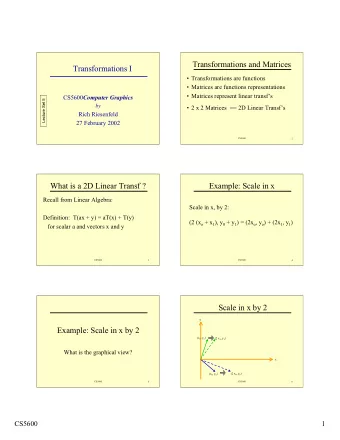
Transforming Points • Geometric transformations modify the spatial relationship between pixels in an image • The images can be shifted, rotated, or stretched in a variety of ways • Geometric transformations can be used to • create thumbnail views • change digital video resolution • correct distortions caused by viewing geometry • align multiple images of the same scene Lin ZHANG, SSE, 2016

Transforming Points Suppose ( w , z ) and ( x , y ) are two spatial coordinate systems input space output space A geometric transformation T that maps the input space to output space    ( , ) ( , ) x y T w z T is called a forward transformation or forward mapping     1 ( , ) ( , ) w z T x y T - 1 is called a inverse transformation or inverse mapping Lin ZHANG, SSE, 2016

Transforming Points    z ( , ) ( , ) x y T w z y     1 ( , ) ( , ) w z T x y x w Lin ZHANG, SSE, 2016

Transforming Points An example     ( , ) ( , ) ( / 2, / 2) x y T w z w z      1 ( , ) ( , ) (2 ,2 ) w z T x y x y Lin ZHANG, SSE, 2016

Contents • Transforming points • Hierarchy of geometric transformations • Applying geometric transformations to images • Image Registration Lin ZHANG, SSE, 2016

Hierarchy of Geometric Transformations • Class I: Isometry transformation If only rotation and translation are considered      '    cos sin   x x t   1             sin cos '      y t   y 2 In homogeneous coordinates   '      cos sin  x t x 1          ' sin cos   y t y     2      1 1 0 0 1    (More concise!)   Lin ZHANG, SSE, 2016

Hierarchy of Geometric Transformations • Class I: Isometry transformation   '      cos sin   x t x     R t x      '    ' x x sin cos    y t y    y 0 1 T         1 1 0 0 1      Properties • R is an orthogonal matrix • Euclidean distance is preserved • Has three degrees of freedom; two for translation, and one for rotation Lin ZHANG, SSE, 2016

Hierarchy of Geometric Transformations • Class II: Similarity transformation   '     cos sin   x s s t x 1     R t   s        ' ' x x sin cos    y s s t y     2 0 1 T        1 1 0 0 1      Lin ZHANG, SSE, 2016

Hierarchy of Geometric Transformations • Class II: Similarity transformation   '     cos sin   x s s t x 1     R t   s        ' ' x x sin cos    y s s t y     2 0 1 T        1 1 0 0 1      Properties • R is an orthogonal matrix • Similarity ratio (the ratio of two lengths) is preserved • Has four degrees of freedom; two for translation, one for rotation, and one for scaling Lin ZHANG, SSE, 2016

Hierarchy of Geometric Transformations • Class III: Affine transformation   '    x a a t x 11 12     A t x       ' ' x x    y a a t y    21 22 y 0 1 T         1 1 0 0 1      Lin ZHANG, SSE, 2016

Hierarchy of Geometric Transformations • Class III: Affine transformation   '    x a a t x 11 12     A t x       ' ' x x    y a a t y    21 22 y 0 1 T         1 1 0 0 1      Properties • A is a non‐singular matrix • Ratio of lengths of parallel line segments is preserved • Has six degrees of freedom; two for translation, one for rotation, one for scaling, one for scaling direction, and one for scaling ratio Lin ZHANG, SSE, 2016

Hierarchy of Geometric Transformations • Class IV: Projective transformation   '    x a a a x 11 12 13        '   c y a a a y     21 22 23      '    z a a a z   31 32 33 Lin ZHANG, SSE, 2016

Hierarchy of Geometric Transformations • Class IV: Projective transformation   '    x a a a x 11 12 13        '   c y a a a y     21 22 23      '    z a a a z   31 32 33 Also referred to as homography matrix Properties • Cross ratio preserved • Though it has 9 parameters, it has 8 degrees of freedom, since only the ratio is important in the homogeneous coordinates Lin ZHANG, SSE, 2016

Contents • Transforming points • Hierarchy of geometric transformations • Applying geometric transformations to images • Image Registration Lin ZHANG, SSE, 2016

Applying Geometric Transformations to Images Given the image f , apply T to f to get g , how to get g ? The procedure for computing the output pixel at location ( x k , y k ) is       1 , ( , ) • Evaluate w z T x y k k k k   , • Evaluate f w z k k      , , • g x y f w z k k k k Lin ZHANG, SSE, 2016

Applying Geometric Transformations to Images • Notes on interpolation ( , ) ( , ) • Even if are integers, in most cases are not x y w z k k k k • For digital images, the values of f are known only at integer‐ valued locations • Using these known values to evaluate f at non‐integer valued locations is called as interpolation z y ( , ) w z k k ( , ) x y k k T  1 x w ( , ) ( , ) g x y f w z Lin ZHANG, SSE, 2016

Applying Geometric Transformations to Images • Notes on interpolation • In Matlab, three commonly used interpolation schemes are built‐in, including nearest neighborhood, bilinear, and bicubic • For most Matlab routines where interpolation is required, “bilinear” is the default Lin ZHANG, SSE, 2016

Applying Geometric Transformations to Images • Matlab implementation • “Maketform” is used to construct a geometric transformation structure • “imtransform” transforms the image according to the 2‐D spatial transformation defined by tform Note: in Matlab, geometric transformations are expressed as   ' 1    ' 1 A x y x y where A is a 3 by 3 transformation matrix Lin ZHANG, SSE, 2016

Applying Geometric Transformations to Images • Matlab implementation An example im = imread('tongji.bmp'); theta = pi/6; rotationMatrix = [cos(theta) sin(theta) 0;-sin(theta) cos(theta) 0;0 0 1]; tformRotation = maketform('affine',rotationMatrix); rotatedIm = imtransform(im, tformRotation,'FillValues',255); figure; subplot(1,2,1); imshow(rotatedIm,[]); rotatedIm = imtransform(im, tformRotation,'FillValues',0); subplot(1,2,2); imshow(rotatedIm,[]); Lin ZHANG, SSE, 2016

Applying Geometric Transformations to Images • Matlab implementation An example original image rotated images Lin ZHANG, SSE, 2016

Applying Geometric Transformations to Images • Matlab implementation Another example original image affine transformed images Lin ZHANG, SSE, 2016

Applying Geometric Transformations to Images • Output image with location specified • This is useful when we want to display the original image and the transformed image on the same figure In Matlab, this is accomplished by imshow(image, ‘XData’, xVector, ‘YData’, yVector) ‘XData’ and ‘YData’ can be obtained by imtransform Lin ZHANG, SSE, 2016

Applying Geometric Transformations to Images • Output image with location specified An example im = imread('tongji.bmp'); theta = pi/4; affineMatrix = [cos(theta) sin(theta) 0;-sin(theta) cos(theta) 0;-300 0 1]; tformAffine = maketform('affine',affineMatrix); [affineIm, XData, YData] = imtransform(im, tformAffine,'FillValues',255); figure; imshow(im,[]); hold on imshow(affineIm,[],'XData',XData,'YData',YData); axis auto axis on Lin ZHANG, SSE, 2016

Applying Geometric Transformations to Images • Output image with location specified An example 0 100 200 300 400 500 600 700 -600 -400 -200 0 200 400 600 Display the original image and the transformed image in the same coordinate system Lin ZHANG, SSE, 2016