Lecture 3: Monte Carlo and Generalization CS234: RL Emma Brunskill - PowerPoint PPT Presentation
Lecture 3: Monte Carlo and Generalization CS234: RL Emma Brunskill Spring 2017 Much of the content for this lecture is borrowed from Ruslan Salakhutdinovs class, Rich Suttons class and David Silvers class on RL. Reinforcement
Lecture 3: Monte Carlo and Generalization CS234: RL Emma Brunskill Spring 2017 Much of the content for this lecture is borrowed from Ruslan Salakhutdinov’s class, Rich Sutton’s class and David Silver’s class on RL.
Reinforcement Learning
Outline • Model free RL: Monte Carlo methods • Generalization • Using linear function approximators • and MDP planning • and Passive RL
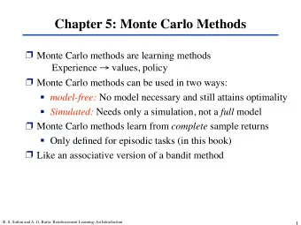
Monte Carlo (MC) Methods ‣ Monte Carlo methods are learning methods - Experience → values, policy ‣ Monte Carlo uses the simplest possible idea: value = mean return ‣ Monte Carlo methods can be used in two ways: - Model-free: No model necessary and still attains optimality - Simulated: Needs only a simulation, not a full model ‣ Monte Carlo methods learn from complete sample returns - Only defined for episodic tasks (this class) - All episodes must terminate (no bootstrapping)
Monte-Carlo Policy Evaluation ‣ Goal: learn from episodes of experience under policy π ‣ Remember that the return is the total discounted reward: ‣ Remember that the value function is the expected return: ‣ Monte-Carlo policy evaluation uses empirical mean return instead of expected return
Monte-Carlo Policy Evaluation ‣ Goal: learn from episodes of experience under policy π ‣ Idea: Average returns observed after visits to s: ‣ Every-Visit MC: average returns for every time s is visited in an episode ‣ First-visit MC: average returns only for first time s is visited in an episode ‣ Both converge asymptotically
First-Visit MC Policy Evaluation ‣ To evaluate state s ‣ The first time-step t that state s is visited in an episode, ‣ Increment counter: ‣ Increment total return: ‣ Value is estimated by mean return ‣ By law of large numbers
Every-Visit MC Policy Evaluation ‣ To evaluate state s ‣ Every time-step t that state s is visited in an episode, ‣ Increment counter: ‣ Increment total return: ‣ Value is estimated by mean return ‣ By law of large numbers
S1 S2 S3 S4 S5 S6 S7 Okay Field Fantastic Site Field Site +1 +10 • Policy: TryLeft (TL) in all states, use ϒ =1, H=4 • Start in state S3, take TryLeft, get r=0, go to S2 • Start in state S2, take TryLeft, get r=0, go to S2 • Start in state S2, take TryLeft, get r=0, go to S1 • Start in state S1, take TryLeft, get r=+1, go to S1 • Trajectory = (S3,TL,0,S2,TL,0,S2,TL,0,S1,TL,1,S1) • First visit MC estimate of S2? • Every visit MC estimate of S2?
Incremental Mean ‣ The mean µ 1 , µ 2 , ... of a sequence x 1 , x 2 , ... can be computed incrementally:
Incremental Monte Carlo Updates ‣ Update V(s) incrementally after episode ‣ For each state S t with return G t ‣ In non-stationary problems, it can be useful to track a running mean, i.e. forget old episodes.
MC Estimation of Action Values (Q) ‣ Monte Carlo (MC) is most useful when a model is not available - We want to learn q*(s,a) ‣ q π (s,a) - average return starting from state s and action a following π ‣ Converges asymptotically if every state-action pair is visited ‣ Exploring starts: Every state-action pair has a non-zero probability of being the starting pair
Monte-Carlo Control ‣ MC policy iteration step: Policy evaluation using MC methods followed by policy improvement ‣ Policy improvement step: greedify with respect to value (or action- value) function
Greedy Policy ‣ For any action-value function q, the corresponding greedy policy is the one that: - For each s, deterministically chooses an action with maximal action-value: ‣ Policy improvement then can be done by constructing each π k+1 as the greedy policy with respect to q π k .
Convergence of MC Control ‣ Greedified policy meets the conditions for policy improvement: ‣ And thus must be ≥ π k. ‣ This assumes exploring starts and infinite number of episodes for MC policy evaluation
Monte Carlo Exploring Starts
On-policy Monte Carlo Control ‣ On-policy: learn about policy currently executing ‣ How do we get rid of exploring starts? - The policy must be eternally soft: π (a|s) > 0 for all s and a. ‣ For example, for ε -soft policy, probability of an action, π (a|s), ‣ Similar to GPI: move policy towards greedy policy ‣ Converges to the best ε -soft policy.
On-policy Monte Carlo Control
Summary so far ‣ MC has several advantages over DP: - Can learn directly from interaction with environment - No need for full models - No need to learn about ALL states (no bootstrapping) - Less harmed by violating Markov property (later in class) ‣ MC methods provide an alternate policy evaluation process ‣ One issue to watch for: maintaining sufficient exploration: - exploring starts, soft policies
Model Free RL Recap • Maintain only V or Q estimates • Update using Monte Carlo or TD-learning • TD-learning • Updates V estimate after each (s,a,r,s’) tuple • Uses biased estimate of V • MC • Unbiased estimate of V • Can only update at the end of an episode • Or some combination of MC and TD • Can use in off policy way • Learn about one policy (generally, optimal policy) • While acting using another
Scaling Up S1 S2 S3 S4 S5 S6 S7 Okay Field Site Fantastic Field +1 Site +10 • Want to be able to tackle problems with enormous or infinite state spaces • Tabular representation is insufficient
Generalization • Don’t want to have to explicitly store a • dynamics or reward model • value • state-action value • policy • for every single state • Want to more compact representation that generalizes
Why Should Generalization Work? • Smoothness assumption • if s 1 is close to s 2 , then (at least one of) • Dynamics are similar, e.g. p(s’|s 1 ,a 1 ) ₎≅ p(s’|s 2 ,a 1 ) • Reward is similar R(s 1 ,a 1 ) ≅ R(s 2 ,a 1 ) • Q functions are similar, Q(s 1 ,a 1 ) ≅ Q(s 2 ,a 1 ) • optimal policy is similar, π ( s 1 ) ≅ π ( s 2 ) • More generally, dimensionality reduction / compression possible • Unnecessary to individually represent each state • Compact representations possible
Benefits of Generalization • Reduce memory to represent T/R/V/Q/policy • Reduce computation to compute V/Q/policy • Reduce experience need to find V/Q/policy
Function Approximation • Key idea: replace lookup table with a function • Today: model-free approaches • Replace table of Q(s,a) with a function • Similar ideas for model-based approaches
Model-free Passive RL: Only maintain estimate of V/Q
Value Function Approximation • Recall: So far V is represented by a lookup table • Every state s has an entry V(s), or • Every state-action pair (s,a) has an entry Q(s,a) • Instead, to scale to large state spaces use function approximation. • Replace table with general parameterized form
Value Function Approximation (VFA) ‣ Value function approximation (VFA) replaces the table with a general parameterized form:
Which Function Approximation? ‣ There are many function approximators, e.g. - Linear combinations of features - Neural networks - Decision tree - Nearest neighbour - Fourier / wavelet bases - … ‣ We consider differentiable function approximators, e.g. - Linear combinations of features - Neural networks
Gradient Descent ‣ Let J(w) be a differentiable function of parameter vector w ‣ Define the gradient of J(w) to be: ‣ To find a local minimum of J(w), adjust w in direction of the negative gradient: Step-size
VFA: Assume Have an Oracle • Assume you can obtain V*(s) for any state s • Goal is to more compactly represent it • Use a function parameterized by weights w
Stochastic Gradient Descent ‣ Goal: find parameter vector w minimizing mean-squared error between the true value function v π (S) and its approximation : ‣ Gradient descent finds a local minimum: ‣ Stochastic gradient descent (SGD) samples the gradient: ‣ Expected update is equal to full gradient update
Feature Vectors ‣ Represent state by a feature vector ‣ For example - Distance of robot from landmarks - Trends in the stock market - Piece and pawn configurations in chess
Linear Value Function Approximation (VFA) ‣ Represent value function by a linear combination of features ‣ Objective function is quadratic in parameters w ‣ Update rule is particularly simple ‣ Update = step-size × prediction error × feature value ‣ Later, we will look at the neural networks as function approximators.
Incremental Prediction Algorithms ‣ We have assumed the true value function v π (s) is given by a supervisor ‣ But in RL there is no supervisor, only rewards ‣ In practice, we substitute a target for v π (s) ‣ For MC, the target is the return G t ‣ For TD(0), the target is the TD target: Remember
VFA for Passive Reinforcement Learning • Recall in passive RL • Following a fixed π • Goal is to estimate V π and/or Q π • In model free approaches • Maintained an estimate of V π / Q π • Used a lookup table for estimate of V π / Q π • Updated it after each step (s,a,s’,r)
Monte Carlo with VFA ‣ Return G t is an unbiased, noisy sample of true value v π (S t ) ‣ Can therefore apply supervised learning to “training data”: ‣ For example, using linear Monte-Carlo policy evaluation ‣ Monte-Carlo evaluation converges to a local optimum
Recommend
More recommend
Explore More Topics
Stay informed with curated content and fresh updates.

