Lecture 2: Introduction to Segmentation Jonathan Krause Fei-Fei Li, - - PowerPoint PPT Presentation

Lecture 2 - Fei-Fei Li, Jonathan Krause 1

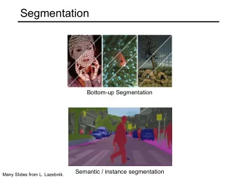
Lecture 2: Introduction to Segmentation

Jonathan Krause

Lecture 2 - Fei-Fei Li, Jonathan Krause

• Goal: Identify groups of pixels that go together

Goal

2

image credit: Steve Seitz, Kristen Grauman

Lecture 2 - Fei-Fei Li, Jonathan Krause

• Semantic Segmentation: Assign labels

Types of Segmentation

3

Tiger Water Grass Dirt

image credit: Steve Seitz, Kristen Grauman

Lecture 2 - Fei-Fei Li, Jonathan Krause

• Figure-ground segmentation: Foreground/background

Types of Segmentation

4

image credit: Carsten Rother

Lecture 2 - Fei-Fei Li, Jonathan Krause

• Co-segmentation: Segment common object

Types of Segmentation

5

image credit: Armand Joulin

Lecture 2 - Fei-Fei Li, Jonathan Krause

Application: As a result

6

Rother et al. 2004

Lecture 2 - Fei-Fei Li, Jonathan Krause

Application: Speed up Recognition

7

Lecture 2 - Fei-Fei Li, Jonathan Krause

Application: Better Classification

8

Angelova and Zhu, 2013

Lecture 2 - Fei-Fei Li, Jonathan Krause

History: Before Computer Vision

9

Lecture 2 - Fei-Fei Li, Jonathan Krause 10

Gestalt Theory

• Gestalt: whole or group

–Whole is greater than sum of its parts –Relationships among parts can yield new properties/features

• Psychologists identified series of factors that predispose

set of elements to be grouped (by human visual system)

“I stand at the window and see a house, trees, sky. 
 Theoretically I might say there were 327 brightnesses 
 and nuances of colour. Do I have "327"? No. I have sky, house, and trees.”

Max Wertheimer


(1880-1943)

Lecture 2 - Fei-Fei Li, Jonathan Krause 11

Gestalt Factors

• These factors make intuitive sense, but are very difficult to translate into algorithms.

Image source: Forsyth & Ponce

Lecture 2 - Fei-Fei Li, Jonathan Krause

• 1. Segmentation as clustering
• 2. Graph-based segmentation
• 3. Segmentation as energy minimization

Outline

12

CS 131 review new stuff

Lecture 2 - Fei-Fei Li, Jonathan Krause

• 1. Segmentation as clustering
• 1. K-Means
• 2. GMMs and EM
• 3. Mean Shift
• 2. Graph-based segmentation
• 3. Segmentation as energy minimization

Outline

13

Lecture 2 - Fei-Fei Li, Jonathan Krause

• Pixels are points in a high-dimensional space
• color: 3d
• color + location: 5d
• Cluster pixels into segments

Segmentation as Clustering

14

Lecture 2 - Fei-Fei Li, Jonathan Krause 15

Clustering: K-Means

Algorithm:

• 1. Randomly initialize the cluster centers, c1, ..., cK
• 2. Given cluster centers, determine points in each cluster
• For each point p, find the closest ci. Put p into cluster i
• 3. Given points in each cluster, solve for ci
• Set ci to be the mean of points in cluster i
• 4. If ci have changed, repeat Step 2
• Properties

– Will always converge to some solution – Can be a “local minimum”

• Does not always find the global minimum of objective function:

slide credit: Steve Seitz

Lecture 2 - Fei-Fei Li, Jonathan Krause

Clustering: K-Means

16

slide credit: Kristen Grauman

k=2 k=3

Lecture 2 - Fei-Fei Li, Jonathan Krause

Clustering: K-Means

17

Note: Visualize segment with average color

Lecture 2 - Fei-Fei Li, Jonathan Krause

Pro:

• Extremely simple
• Efficient

Con:

• Hard quantization in clusters
• Can’t handle non-spherical

clusters

K-Means

18

Lecture 2 - Fei-Fei Li, Jonathan Krause

• Represent data distribution as mixture of

multivariate Gaussians.

Gaussian Mixture Model

19

How do we actually fit this distribution?

Lecture 2 - Fei-Fei Li, Jonathan Krause 20

Expectation Maximization (EM)

• Goal

– Find parameters θ (for GMMs: ) that maximize the likelihood function:

• Approach:
• 1. E-step: given current parameters, compute ownership of each point
• 2. M-step: given ownership probabilities, update parameters to maximize

likelihood function

• 3. Repeat until convergence

See CS229 material if this is unfamiliar!

Lecture 2 - Fei-Fei Li, Jonathan Krause

Clustering: Expectation Maximization (EM)

21

Lecture 2 - Fei-Fei Li, Jonathan Krause

Pro:

• Still fairly simple and efficient
• Model more complex distributions

Con:

• Need to know number of components in

advance — hard to know unless you’re looking at the data yourself!

GMMs

22

Lecture 2 - Fei-Fei Li, Jonathan Krause 23

Clustering: Mean-shift

• 1. Initialize random seed, and window W
• 2. Calculate center of gravity (the “mean”) of W:
• Can generalize to arbitrary windows/kernels
• 3. Shift the search window to the mean
• 4. Repeat Step 2 until convergence

slide credit: Steve Seitz

Only parameter: window size

Fei-Fei Li, Jonathan Krause

Lecture 2 -

Mean-Shift

24

Region of interest Center of mass Mean Shift vector

Slide by Y . Ukrainitz & B. Sarel

Fei-Fei Li, Jonathan Krause

Lecture 2 -

Region of interest Center of mass Mean Shift vector

Mean-Shift

25

Slide by Y . Ukrainitz & B. Sarel

Fei-Fei Li, Jonathan Krause

Lecture 2 -

Region of interest Center of mass Mean Shift vector

Mean-Shift

26

Slide by Y . Ukrainitz & B. Sarel

Fei-Fei Li, Jonathan Krause

Lecture 2 -

Region of interest Center of mass

Mean-Shift

27

Slide by Y . Ukrainitz & B. Sarel

Lecture 2 - Fei-Fei Li, Jonathan Krause 28

Clustering: Mean-shift

slide credit: Y. Ukrainitz & B. Sarel

• Cluster: all data points in the attraction basin of a mode
• Attraction basin: the region for which all trajectories

lead to the same mode

Lecture 2 - Fei-Fei Li, Jonathan Krause 29

Mean-shift for segmentation

• Find features (color, gradients, texture, etc)
• Initialize windows at individual pixel locations
• Perform mean shift for each window until convergence
• Merge windows that end up near the same “peak” or mode

Lecture 2 - Fei-Fei Li, Jonathan Krause

Mean-shift for segmentation

30

Lecture 2 - Fei-Fei Li, Jonathan Krause

Pro:

• No number of clusters assumption
• Handle unusual distributions
• Simple

Con:

• Choice of window size
• Can be somewhat expensive

Mean Shift

31

Lecture 2 - Fei-Fei Li, Jonathan Krause

Pro:

• Generally simple
• Can handle most data distributions

with sufficient effort.

Con:

• Hard to capture global structure
• Performance is limited by

simplicity

Clustering

32

Lecture 2 - Fei-Fei Li, Jonathan Krause

• 1. Segmentation as clustering
• 2. Graph-based segmentation
• 1. General Properties
• 2. Spectral Clustering
• 3. Min Cuts
• 4. Normalized Cuts
• 3. Segmentation as energy minimization

Outline

33

Lecture 2 - Fei-Fei Li, Jonathan Krause 34

Images as Graphs

– Node (vertex) for every pixel – Edge between pairs of pixels, (p,q) – Affinity weight wpq for each edge

• wpq measures similarity
• Similarity is inversely proportional to difference 


(in color and position…)

q p wpq

w

slide credit: Steve Seitz

Lecture 2 - Fei-Fei Li, Jonathan Krause 35

Images as Graphs

Which edges to include? Fully connected:

• Captures all pairwise similarities
• Infeasible for most images

Neighboring pixels:

• Very fast to compute
• Only captures very local interactions

Local neighborhood:

• Reasonably fast, graph still very sparse
• Good tradeoff

w

Lecture 2 - Fei-Fei Li, Jonathan Krause 36

Measuring Affinity

• In general:
• Examples:
• Distance:
• Intensity:
• Color:
• Texture:
• Note: Can also modify distance metric

slide credit: Forsyth & Ponce

Lecture 2 - Fei-Fei Li, Jonathan Krause 37

Measuring Affinity

Distance:

slide credit: Forsyth & Ponce

Lecture 2 - Fei-Fei Li, Jonathan Krause 38

Measuring Affinity

Intensity:

slide credit: Forsyth & Ponce

Lecture 2 - Fei-Fei Li, Jonathan Krause 39

Measuring Affinity

Color:

slide credit: Forsyth & Ponce

Lecture 2 - Fei-Fei Li, Jonathan Krause 40

Measuring Affinity

Texture:

slide credit: Forsyth & Ponce

Lecture 2 - Fei-Fei Li, Jonathan Krause 41

Segmentation as Graph Cuts

• Break Graph into Segments

– Delete links that cross between segments – Easiest to break links that have low similarity (low weight)

• Similar pixels should be in the same segments
• Dissimilar pixels should be in different segments

w A B C

slide credit: Steve Seitz

Lecture 2 - Fei-Fei Li, Jonathan Krause

• Given: Affinity matrix W
• Goal: Extract a single good cluster v
• v(i): score for point i for cluster v

Graph Cut with Eigenvalues

42

Lecture 2 - Fei-Fei Li, Jonathan Krause

Optimizing

43

Lagrangian: v is an eigenvector of W

Lecture 2 - Fei-Fei Li, Jonathan Krause

• 1. Construct affinity matrix W
• 2. Compute eigenvalues and vectors of W
• 3. Until done

1. Take eigenvector of largest unprocessed eigenvalue 2. Zero all components of elements that have already been clustered 3. Threshold remaining components to determine cluster membership Note: This is an example of a spectral clustering algorithm

Clustering via Eigenvalues

44

Lecture 2 - Fei-Fei Li, Jonathan Krause 45

Graph Cuts - Another Look

• Set of edges whose removal makes a graph disconnected
• Cost of a cut

– Sum of weights of cut edges:

• A graph cut gives us a segmentation

– What is a “good” graph cut and how do we find one?

A B

slide credit: Steve Seitz

Lecture 2 - Fei-Fei Li, Jonathan Krause

• We can do segmentation by finding the minimum cut
• either smallest number of elements (unweighted) or

smallest sum of weights (weighted)

• efficient algorithms exist
• Drawback
• Weight of cut proportional to number of edges
• Biased towards cutting small, isolated components

Formulation: Min Cut

46

Ideal Cut Cuts with lesser weight than the ideal cut

image credit: Khurran Hassan-Shafique

Lecture 2 - Fei-Fei Li, Jonathan Krause

• Key idea: normalize segment size
• Fixes min cut’s bias
• Formulation:
• NP-hard, but can approximate

Formulation: Normalized Cuts

47

) , ( ) , ( ) , ( ) , ( V B assoc B A cut V A assoc B A cut +

= sum of weights of edges in V that touch A

• J. Shi and J. Malik. Normalized cuts and image segmentation. PAMI 2000

Lecture 2 - Fei-Fei Li, Jonathan Krause 48

NCuts as Generalized Eigenvector Problem

Slide credit: Jitendra Malik

Definitions: In matrix form: : affinity matrix : diagonal matrix : vector in

Lecture 2 - Fei-Fei Li, Jonathan Krause 49

After a lot of math…

• After simplification, we get
• This is a Rayleigh Quotient

– Solution given by the “generalized” eigenvalue problem

• Subtleties

– Optimal solution is second smallest eigenvector – Gives continuous result—must convert into discrete values of y

Slide credit: Alyosha Efros

This is hard,
 y is discrete! Relaxation:
 continuous y

Lecture 2 - Fei-Fei Li, Jonathan Krause

NCuts example

50

Smallest eigenvectors

Image source: Shi & Malik

NCuts segments

Lecture 2 - Fei-Fei Li, Jonathan Krause

• 1. Construct weighted graph
• 2. Construct affinity matrix
• 3. Solve for smallest few

eigenvectors.

• This is a continuous solution
• 4. Threshold eigenvectors to get a discrete cut
• This is the approximation
• As before, several heuristics for doing this
• 5. Recursively subdivide as desired.

NCuts: Algorithm Summary

51

Lecture 2 - Fei-Fei Li, Jonathan Krause

NCuts examples

52

Lecture 2 - Fei-Fei Li, Jonathan Krause

NCuts examples

53

Lecture 2 - Fei-Fei Li, Jonathan Krause

• Pro
• Flexible to choice of affinity matrix
• Generally works better than other

methods we’ve seen so far

• Con
• Can be expensive, especially with many

cuts.

• Bias toward balanced partitions
• Constrained by affinity matrix model

NCuts Pro and Con

54

Slide source: Kristen Grauman

Lecture 2 - Fei-Fei Li, Jonathan Krause

• 1. Segmentation as clustering
• 2. Graph-based segmentation
• 3. Segmentation as energy minimization
• 1. MRFs + CRFs
• 2. Segmentation with CRFs
• 3. GrabCut

Outline

55

Lecture 2 - Fei-Fei Li, Jonathan Krause

• Rich probabilistic model for images
• Built in local, modular way
• Get global effects from only learning/modeling local
• nes
• After conditioning, get a Markov Random Field (MRF)

Conditional Random Fields (CRFs)

56

Observed evidence Hidden “true states” Neighborhood relations

x1 x3 x2 x4 y4 y2 y3 y1

Lecture 2 - Fei-Fei Li, Jonathan Krause

Pixels as CRF Nodes

57 Reconstruction
 from MRF modeling
 pixel neighborhood 
 statistics Degraded image Original image

Image source: Bastian Liebe

Lecture 2 - Fei-Fei Li, Jonathan Krause

CRF Probability

58

Scene Image Image-scene compatibility function Local

• bservations

Scene-scene compatibility function Neighboring scene nodes Partition Function

Lecture 2 - Fei-Fei Li, Jonathan Krause 59

Energy Formulation

take logs, drop

• We call an energy function
• named from free-energy problems in statistical mechanics
• Individual terms are potentials
• Note: Derived this way, it’s energy maximization. Be

careful and check each formulation individually.

Lecture 2 - Fei-Fei Li, Jonathan Krause

• Unary potentials 𝜒
• Local information about each pixel
• e.g. how likely a pixel/patch belongs to a certain class
• Pairwise potentials ψ
• Neighborhood information, enforces consistency
• e.g. how different a pixel is from its neighbor in

appearance

Energy Formulation

60

slide credit: Bastian Liebe

Lecture 2 - Fei-Fei Li, Jonathan Krause

• Boykov and Jolly (2001)
• Variables
• xi : Annotation (Input)
• Foreground/background/empty
• yi : Binary variable
• Foreground/background
• Unary term
• Penalty for disregarding annotation
• Pairwise term
• Encourage smooth annotations
• wij is affinity between pixels i and j

CRF segmentation example

61

Lecture 2 - Fei-Fei Li, Jonathan Krause

• Grid structured random fields
• Maxflow/mincut
• Optimal for binary labeling
• submodular energy functions
• Boykov & Kolmogorov, “An

Experimental Comparison of Min- Cut/Max-Flow Algorithms for Energy Minimization in Vision”, PAMI 2004

• Fully connected models
• Efficient solution with convolution

mean-field

• Krähenbühl and Koltun, “Efficient

Inference in Fully-Connected CRFs with Gaussian Edge Potentials”, NIPS 2011

Solving Efficiently

62

Lecture 2 - Fei-Fei Li, Jonathan Krause

GrabCut: Interactive Foreground Extraction

63

Lecture 2 - Fei-Fei Li, Jonathan Krause

• Variables
• xi: pixel
• yi ∈ {0,1}: foreground/background label {0,1}
• ki ∈ {0, …, K-1}: GMM mixture component
• θ: GMM model parameters
• I = {z1, …, zm}: RGB image
• Unary Term
• log of GMM probability
• Pairwise Term

GrabCut formulation

64

Lecture 2 - Fei-Fei Li, Jonathan Krause

• 1. Initialize Mixture Models based on user annotation
• 2. Assign GMM components
• 3. Learn GMM parameters
• 4. Estimate segmentations (mincut)
• 5. Repeat 2-4 until convergence

GrabCut - Iterative Optimization

65

Lecture 2 - Fei-Fei Li, Jonathan Krause

GrabCut results

66

Lecture 2 - Fei-Fei Li, Jonathan Krause

Further editing with GrabCut

67

Lecture 2 - Fei-Fei Li, Jonathan Krause

• Pros
• Very powerful, get global results by defining local

interactions

• Very general
• Rather efficient
• Becoming more or less standard for many segmentation

problems (GrabCut was 2004!)

• Cons
• Only works for sub modular energy functions (binary)
• Only approximate algorithms work for multi-label case

Summary: Graph Cuts with CRFs

68

Lecture 2 - Fei-Fei Li, Jonathan Krause

• Images contain a lot of pixels
• Even efficient methods can be slow
• Efficiency trick: Superpixels
• Group together similar pixels
• Cheap and local over segmentation
• Must be high precision!
• Many methods exist, try several.
• Another trick: Resize the image
• Do segmentation in lower-res version,

then scale back up to high-res.

Extra: Improving Segmentation Efficiency

69

Lecture 2 - Fei-Fei Li, Jonathan Krause

• CS 131/CS231a slides (all)
• CS 229 (clustering, EM)
• CS 228/228T (MRFs, CRFs, energy minimization)
• EE 364 (optimization)

Additional Reading

70