Lecture 18: Recognition IV Thursday, Nov 15 Prof. Kristen Grauman - - PDF document

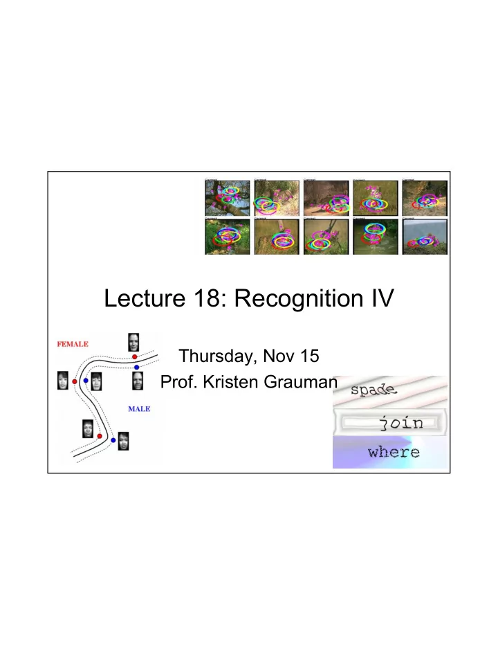
Lecture 18: Recognition IV

Thursday, Nov 15

• Prof. Kristen Grauman

Outline

• Discriminative classifiers

– SVMs

• Learning categories from weakly supervised images

– Constellation model

• Shape matching

– Shape context, visual CAPTCHA application

Recall: boosting

• Want to select the single feature that best

separates positive and negative examples, in terms of weighted error.

Each dimension: output of a possible rectangle feature

• n faces and non-faces.

Recall: boosting

• Want to select the single feature that best

separates positive and negative examples, in terms of weighted error.

Each dimension: output of a possible rectangle feature

• n faces and non-faces.

=

Recall: boosting

• Want to select the single feature that best

separates positive and negative examples, in terms of weighted error.

Each dimension: output of a possible rectangle feature

• n faces and non-faces.

Image subwindow Optimal threshold that results in minimal misclassifications = Notice that any threshold giving same error rate would be equally good here.

Lines in R2

= + + d by ax

Lines in R2

⎥ ⎦ ⎤ ⎢ ⎣ ⎡ = b a w ⎥ ⎦ ⎤ ⎢ ⎣ ⎡ = y x x

= + + d by ax

Let

Lines in R2

= + ⋅ d x w

⎥ ⎦ ⎤ ⎢ ⎣ ⎡ = b a w ⎥ ⎦ ⎤ ⎢ ⎣ ⎡ = y x x

= + + d by ax

Let

w

Lines in R2

= + ⋅ d x w

⎥ ⎦ ⎤ ⎢ ⎣ ⎡ = b a w ⎥ ⎦ ⎤ ⎢ ⎣ ⎡ = y x x

= + + d by ax

Let

w

( )

0, y

x

D

Lines in R2

= + ⋅ d x w

⎥ ⎦ ⎤ ⎢ ⎣ ⎡ = b a w ⎥ ⎦ ⎤ ⎢ ⎣ ⎡ = y x x

= + + d by ax

Let

w

( )

0, y

x

D w x w d b a d by ax D + = + + + =

Τ 2 2

distance from point to line

Lines in R2

= + ⋅ d x w

⎥ ⎦ ⎤ ⎢ ⎣ ⎡ = b a w ⎥ ⎦ ⎤ ⎢ ⎣ ⎡ = y x x

= + + d by ax

Let

w

( )

0, y

x

D w x w d b a d by ax D + = + + + =

Τ 2 2

distance from point to line

Planes in R3

= + + + d cz by ax

= + ⋅ d x w

⎥ ⎥ ⎥ ⎦ ⎤ ⎢ ⎢ ⎢ ⎣ ⎡ = c b a w ⎥ ⎥ ⎥ ⎦ ⎤ ⎢ ⎢ ⎢ ⎣ ⎡ = z y x x

Let

w

w x w d c b a d cz by ax D + = + + + + + =

Τ 2 2 2

distance from point to plane

( )

, , z y x

D

Hyperplanes in Rn

2 2 1 1

= + + + + b x w x w x w

n n

K

Hyperplane H is set of all vectors which satisfy:

n

R ∈ x

= +

Τ

b x w

w x w x b H D + =

Τ

) , (

distance from point to hyperplane

Support Vector Machines (SVMs)

• Discriminative

classifier based on

• ptimal separating

hyperplane

• What hyperplane is
• ptimal?

Linear Classifiers

f

x

yest

denotes + 1 denotes -1

f(x,w,b) = sign(w x + b)

How would you classify this data?

w x + b=0 w x + b<0 w x + b>0 Slides from Andrew Moore’s tutorial: http://www.autonlab.org/tutorials/svm.html

Linear Classifiers

f

x

yest

denotes + 1 denotes -1

f(x,w,b) = sign(w x + b)

How would you classify this data?

Linear Classifiers

f

x

yest

denotes + 1 denotes -1

f(x,w,b) = sign(w x + b)

How would you classify this data?

Linear Classifiers

f

x

yest

denotes + 1 denotes -1

f(x,w,b) = sign(w x + b)

Any of these would be fine.. ..but which is best?

Linear Classifiers

f

x

yest

denotes + 1 denotes -1

f(x,w,b) = sign(w x + b)

How would you classify this data?

Misclassified to +1 class

Classifier Margin

f

x

yest

denotes + 1 denotes -1

f(x,w,b) = sign(w x + b)

Define the margin

• f a linear

classifier as the width that the boundary could be increased by before hitting a datapoint.

Classifier Margin

f

x

yest

denotes + 1 denotes -1

f(x,w,b) = sign(w x + b)

Define the margin

• f a linear

classifier as the width that the boundary could be increased by before hitting a datapoint.

Maximum Margin

f

x

yest

denotes + 1 denotes -1

f(x,w,b) = sign(w x + b)

The maximum margin linear classifier is the linear classifier with maximum margin. This is the simplest kind of SVM (Called an LSVM)

Linear SVM Support Vectors are those datapoints that the margin pushes up against 1. Maximizing the margin is good according to intuition and theory 2. Implies that only support vectors are important; other training examples are ignorable. 3. Empirically it works very very well.

Linear SVM Mathematically

“ P r e d i c t C l a s s = + 1 ” z

• n

e “ P r e d i c t C l a s s =

• 1

” z

• n

e

wx+ b= 1 wx+ b= 0 wx+ b= -1

X- x+

M= Margin Width

w w w 2 1 1 = − − = M

w w x w 1 ± = + b

Τ

For the support vectors, distance to hyperplane is 1 for a positives and -1 for negatives.

Question

• How should we choose values for w,b?

1.want the training data separated by the hyperplane so it classifies them correctly 2.want the margin width M as large as possible

Linear SVM Mathematically

Goal: 1) Correctly classify all training data

if yi = +1 if yi = -1 for all i

2) Maximize the Margin same as minimize

• Formulated as a Quadratic Optimization Problem, solve for w and b:

Minimize

subject to w M 2 =

w w w

t

2 1 ) ( = Φ

1 ≥ + b wx i

1 ≤ + b wx i

1 ) ( ≥ + b wx y

i i

1 ) ( ≥ + b wx y

i i

i ∀

w wt 2 1

The Optimization Problem Solution

Solution has the form (omitting derivation): Each non-zero αi indicates that corresponding xi is a

support vector.

Then the classifying function will have the form: Notice that it relies on an inner product between the test

point x and the support vectors xi

Solving the optimization problem also involves

computing the inner products xi

Txj between all pairs of

training points.

w =Σαiyixi b= yk- wTxk for any xk such that αk≠ 0 f(x) = Σαiyixi

Tx + b

Non-linear SVMs

Datasets that are linearly separable with some noise

work out great:

But what are we going to do if the dataset is just too hard? How about… mapping data to a higher-dimensional

space:

x x x x2

Non-linear SVMs: Feature spaces

General idea: the original input space can always be

mapped to some higher-dimensional feature space where the training set is separable:

Φ: x → φ(x)

The “Kernel Trick”

• The linear classifier relies on dot product between vectors K(xi,xj)=xi

Txj

• If every data point is mapped into high-dimensional space via some

transformation Φ: x → φ(x), the dot product becomes: K(xi,xj)= φ(xi) Tφ(xj)

• A kernel function is similarity function that corresponds to an inner product

in some expanded feature space.

• Example:

2-dimensional vectors x=[x1 x2]; let K(xi,xj)=(1 + xi

Txj)2

Need to show that K(xi,xj)= φ(xi) Tφ(xj): K(xi,xj)=(1 + xi

Txj)2 ,

= 1+ xi1

2xj1 2 + 2 xi1xj1 xi2xj2+ xi2 2xj2 2 + 2xi1xj1 + 2xi2xj2

= [1 xi1

2 √2 xi1xi2 xi2 2 √2xi1 √2xi2]T [1 xj1 2 √2 xj1xj2 xj2 2 √2xj1 √2xj2]

= φ(xi) Tφ(xj), where φ(x) = [1 x1

2 √2 x1x2 x2 2 √2x1 √2x2]

Examples of General Purpose Kernel Functions

Linear: K(xi,xj)= xi Txj

Polynomial of power p: K(xi,xj)= (1+ xi Txj)p Gaussian (radial-basis function network):

) 2 exp( ) , (

2 2

σ

j i j i

x x x x − − = K

SVMs for object recognition

• 1. Define your representation

for each example.

• 2. Select a kernel function.
• 3. Compute pairwise kernel

values between labeled examples, identify support vectors.

• 4. Compute kernel values

between new inputs and support vectors to classify.

Example: learning gender with SVMs

Moghaddam and Yang, Learning Gender with Support Faces, TPAMI 2002. Moghaddam and Yang, Face & Gesture 2000.

Moghaddam and Yang, Learning Gender with Support Faces, TPAMI 2002.

Processed faces Face alignment processing

• Training examples:

– 1044 males – 713 females

• Experiment with various kernels, select

Gaussian RBF

Learning gender with SVMs

Support Faces

Moghaddam and Yang, Learning Gender with Support Faces, TPAMI 2002.

Moghaddam and Yang, Learning Gender with Support Faces, TPAMI 2002.

Gender perception experiment: How well can humans do?

• Subjects:

– 30 people (22 male, 8 female) – Ages mid-20’s to mid-40’s

• Test data:

– 254 face images (6 males, 4 females) – Low res and high res versions

• Task:

– Classify as male or female, forced choice – No time limit

Moghaddam and Yang, Face & Gesture 2000.

Moghaddam and Yang, Face & Gesture 2000.

Gender perception experiment: How well can humans do?

Error Error

Human vs. Machine

• SVMs

perform better than any single human text subject

Hardest examples for humans

Moghaddam and Yang, Face & Gesture 2000.

Summary: SVM classifiers

• Discriminative classifier
• Effective for high-dimesional data
• Flexibility/modularity due to kernel
• Very good performance in practice, widely

used in vision applications

Outline

• Discriminative classifiers

– SVMs

• Learning categories from weakly supervised images

– Constellation model

• Shape matching

– Shape context, visual CAPTCHA application

Weak supervision

• How can we learn object models in the

presence of clutter?

Vs.

Goal

Slide from Li Fei-Fei http://www.vision.caltech.edu/feifeili/Resume.htm

• Questions:

– What about categories where an iconic “template” representation is infeasible? – What is the object to be recognized / the part

• f the image we want to build a model for?

– For that object, what parts are distinctive or things that can be reliably detected in different instances?

Weak supervision

Weber, Welling, Perona. Unsupervised Learning of Models for Recognition, ECCV 2000.

Weber, Welling, Perona., 2000.

Slide by Bill Freeman, MIT

Slide by Bill Freeman, MIT

Slide by Bill Freeman, MIT

Slide by Bill Freeman, MIT

Slide by Bill Freeman, MIT

Part-based models

Part-based models

Slide by Fei-Fei Li, 2003.

One possible constellation model

• Model class with joint probability density

function on shape and appearance

Figure from Rob Fergus

image patch descriptors, with uncertainty mutual positions of the parts, with uncertainty

Unsupervised learning of part- based models

Main idea:

• Use interest operator to detect small highly textured

regions (on both fg and bg) – If training objects have similar appearance, these regions will often be similar in different training examples

• Cluster patches: large clusters used to select candidate

fg parts

• Choose most informative parts while simultaneously

estimating model parameters – Iteratively try different combinations of a small number of parts and check model performance on validation set to evaluate quality

Weber, Welling, Perona, ECCV 2000.

Representation

• Use a scale invariant, scale sensing feature keypoint

detector (like the first steps of Lowe’s SIFT).

From: Rob Fergus http://www.robots.ox.ac.uk/%7Efergus/

Features Keys

• A direct appearance model is taken around each located
• key. This is then normalized to an 11x11 window. PCA

further reduces these features.

From: Rob Fergus http://www.robots.ox.ac.uk/%7Efergus/

Slide by Bill Freeman, MIT

Candidate parts

Weber, Welling, Perona. Unsupervised Learning of Models for Recognition, 2000.

For faces For cars At this point, parts appear in both background and foreground of training images.

Model learning

Images from Rob Fergus

Which of the candidate parts define the class, and in what configuration? Let’s assume:

• We know number of parts that define the

model (and can keep it small).

• Object of interest is only consistent thing

somewhere in each training image.

Model learning

Which of the candidate parts define the class, and in what configuration? Initialize model parameters randomly. Iterate while fit improves:

• 1. Find best assignment in the

training images given the parameters

• 2. Recompute parameters

based on current features

Recognition

• Given a model defining the object class and a

model for “background”, compute likelihood ratio to make Bayesian decision:

X: locations S: scales A: appearances

Identified in new image:

Recognition

• Given a model defining the object class and a

model for “background”, compute likelihood ratio to make Bayesian decision:

X: locations S: scales A: appearances Use maximum-likelihood parameters

Example: data from four categories

Slide from Li Fei-Fei http://www.vision.caltech.edu/feifeili/Resume.htm

Face model Recognition results Appearance: 10 patches closest to mean for each part

Face model Recognition results Appearance: 10 patches closest to mean for each part

Appearance: 10 patches closest to mean for each part Motorbike model Recognition results

Appearance: 10 patches closest to mean for each part Spotted cat model Recognition results

Outline

• Discriminative classifiers

– SVMs

• Learning categories from weakly supervised images

– Constellation model

• Shape matching

– Shape context, visual CAPTCHA application

Shape and biology

• D’Arcy Thompson: On Growth and Form, 1917

– studied transformations between shapes of

• rganisms

Slides adapted from Belongie, Malik, & Puzicha, Matching Shapes, ICCV 2001. www.eecs.berkeley.edu/Research/Projects/CS/vision/shape/belongie-iccv01

Shape matching for recognition

model target

Comparing shapes

What points on these two sampled contours are most similar?

Shape context descriptor

Count the number of points inside each bin, e.g.: Count = 4 Count = 10 ... Compact representation

• f distribution of points

relative to each point

Shape context descriptor

Comparing shape contexts

Compute matching costs using Chi Squared distance: Recover correspondences by solving for least cost assignment, using costs Cij (Then estimate a parameterized transformation based on these correspondences.)

CAPTCHA’s

• CAPTCHA: Completely Automated Turing Test

To Tell Computers and Humans Apart

• Luis von Ahn, Manuel Blum, Nicholas Hopper

and John Langford, CMU, 2000.

• www.captcha.net

Shape matching application: breaking a visual CAPTCHA

• Use shape matching to recognize characters,

words in spite of clutter, warping, etc.

Recognizing Objects in Adversarial Clutter: Breaking a Visual CAPTCHA, by G. Mori and J. Malik, CVPR 2003

Computer Vision Group

University of California

Berkeley

Fast Pruning: Representative Shape Contexts

• Pick k points in the image at random

– Compare to all shape contexts for all known letters – Vote for closely matching letters

• Keep all letters with scores under threshold

d

• p

Slides by Greg Mori, CVPR 2003

Computer Vision Group

University of California

Berkeley

Algorithm A: bottom-up

• Look for letters

– Representative Shape Contexts

• Find pairs of letters that

are “consistent”

– Letters nearby in space

• Search for valid words
• Give scores to the words

Computer Vision Group

University of California

Berkeley

EZ-Gimpy Results with Algorithm A

• 158 of 191 images correctly identified: 83%

– Running time: ~10 sec. per image (MATLAB, 1 Ghz P3) horse smile canvas spade join here

Computer Vision Group

University of California

Berkeley

Gimpy

• Multiple words, task is to find 3 words in the

image

• Clutter is other objects, not texture

Computer Vision Group

University of California

Berkeley

Algorithm B: Letters are not enough

• Hard to distinguish single letters with so much clutter
• Find words instead of letters

– Use long range info over entire word – Stretch shape contexts into ellipses

• Search problem becomes huge

– # of words 600 vs. # of letters 26 – Prune set of words using opening/closing bigrams

Computer Vision Group

University of California

Berkeley

Results with Algorithm B

# Correct words % tests (of 24) 1 or more 92% 2 or more 75% 3 33% EZ-Gimpy 92%

dry clear medical door farm important card arch plate

Coming up

• Face images
• For next week:

– Read Trucco & Verri handout on Motion

• Problem set 4 due 11/29

References

• Unsupervised Learning of Models for Recognition, by M.

Weber, M. Welling and P. Perona, ECCV 2000.

• Towards Automatic Discovery of Object Categories, by
• M. Weber, M. Welling and P. Perona, CVPR 2000.
• Object Class Recognition by Unsupervised Scale-

Invariant Learning, by Fergus, Perona, and Zisserman, CVPR 2003.

• Matching Shapes, by S. Belongie, J. Malik and J.

Puzicha, ICCV 2001.

• Recognizing Objects in Adversarial Clutter: Breaking a

Visual CAPTCHA, by G. Mori and J. Malik, CVPR 2003.

• Learning Gender with Support Faces, by Moghaddam

and Yang, TPAMI, 2002.

• SVM slides from Andrew Moore, CMU